Yanán Camaraza-Medina* | Andres A. Sánchez-Escalona | Yoalbys Retirado-Mediaceja | Osvaldo F. García-Morales
© 2020 IIETA. This article is published by IIETA and is licensed under the CC BY 4.0 license (http://creativecommons.org/licenses/by/4.0/).
OPEN ACCESS
In the present times, the use of air cooled condenser (ACC) has become generalized where the installation of power plants is required and access to condensation water is difficult. At present it is known that performing the thermal evaluation of an ACC is a complex task, since the existing methods do not consider all the elements that directly influence the performance of the ACC. A very widespread method is that attributed to Kröger, however its use does not provide adequate results for high values of environmental temperature, which is a limitation to be applied in tropical countries like Cuba. This document provides an analysis method that includes the effect of environmental variables and that allows reasonable results to be obtained for high values of ambient temperature. The new proposal follows the logical sequence of the Kröger method, but considering a new procedure for the determination of the mean heat transfer coefficients and pressure drops, required for the thermal evaluation of ACC.
efficiency, power plant, sugar industry, heat transfer
In the present times, the low availability of water and the urgent need to use renewable energy sources, have resulted in an important group of contributions aimed at solving the deficiencies that emerging technologies present. Biomass as a source of energy for the generation of electrical power has been one of the solutions used and most widely accepted in countries and regions with ease of access to biomass resources, [1, 2].
Dry condensers, including the air cooled condenser (ACC), are an alternative widely used today to reduce water consumption in biomass power plants (BPP). The ACC and dry condensers make it possible to significantly reduce the use of water intended for condensation, requiring only 5% of the volume required by conventional wet condensers. Of the dry condensers, ACC is the most widely used in BPP facilities. At present it finds application in facilities that are operating in countries such as China, South Africa, Spain and Turkey [3].
Cuba is not exempt from the global energy crisis. To deal with this problem, a strategy has been drawn up for the five-year period (2020-2025) which includes an investment that will complete the installation and start-up of a group of facilities for the generation of electricity from the use of renewable sources of energy (1,650 MW). This generation volume constitutes approximately 24% of the country's energy needs. This project includes a total of 25 BPP linked to sugar processing plants (SPP), which will be in charge of supplying the bagasse used as fuel in the BPP, while BPP will supply the steam required by SPP's industrial process [4].
In Cuba, studies carried out by the entity in charge of the regulation and use of water, have shown that the proven water deficit has grown rapidly, reaching 12% at the end of 2019, with a total of 60 watersheds being declared in a depressed state of its heights. To face this situation, laws 24/2017 and 337/2017 were enacted that regulate the use of water. Of the 25 planned BPPs, a total of 17 are located in areas of operation with a deficit of access to water, so the use of ACC can be an effective solution for the start-up of these facilities. Cuba is not distant of the global crisis of water, therefore, it is essential to give an adequate use, this has motivated that has been considered to medium term the use of technology ACC in the projects planned of BPP [5].
Performing the thermal analysis of an ACC is a complex and difficult task to execute. Modern Engineering does not have a single procedure to carry out the thermal and hydraulic study of an ACC, which brings together all the elements that influence its efficiency and its subsequent effect on the operation of the BPP.
A method considered effective in the literature consulted and available is that attributed to Kröger, however, it has as a fundamental limitation that the precision of the results obtained with its use is penalized with the increase in dry bulb temperature (TTBS). The tropical climate of Cuba generates that in almost the entire year there are high values of TTBS, which is an important impediment to extend its use to the BPP project, because the results obtained can compute dispersion values close to 60 % [6, 7].
With the firm purpose of developing a unique method that allows evaluating the performance of an ACC, the authors pursue as the main objective of this study, to bring together in a single analysis procedure, a method that includes the direct effect of environmental variables and more precise and less dispersed than currently available procedures. This research is part of the postdoctoral studies carried out by the main author.
2.1 Basic methodology for the selection of the more adequate condenser
In order to choose the most suitable condensing system, it is necessary to take into consideration an important group of elements. For this purpose, a methodology is elaborated which is presented in the form of a selection diagram (see Figure 1). The selection of the condensation system requires having a primary group of input data, which are summarized in Table 1. The quick selection graph is an alternative for the quick choice of operating parameters for pre-established conditions of the TPP, this method is a quick and moderately effective, but allow to obtain the effectiveness of the ACC in a first intend [5].
Figure 1. Basic procedure for condenser selection
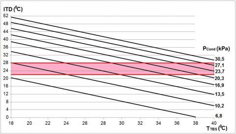
Diagram of the temperature variation is a rapid solution for the selection of most adequate operation intervals in the ACC, (see Figure 2). In diagram of the temperature variation, an interaction between the initial temperature difference (ITD) and the temperature of dry bulb (TTBS) are shown, in terms of the steam pressure in the turbine outlet (PCond). The zone recommended of favorable operation was obtained in recent investigations, in this paper being is highlighted in pink color (see Figure 2) [8].
A very important element in the thermal evaluation of an ACC is the initial temperatures difference (ITD), which can be described as [8]:
$\mathrm{ITD}=\mathrm{T}_{\mathrm{EntVapor}}-\mathrm{T}_{\mathrm{TBS}}$ (1)
where:
$\mathrm{T}_{\text {EntVapor }}$ - Fluid temperature in the ACC inlet, in ℃.
Table 1. Required variables for thermal evaluation
|
- |
Water availability to be used in the condenser |
|
$P_{C}$ |
Capacity of the power plant, in MW |
|
- |
Cost of the water use, in $\mathrm{USD} / \mathrm{m}^{3}$ |
|
- |
Altitude above sea level |
|
$\mathrm{h}_{\mathrm{rel}}$ |
Relative humidity, in %. |
|
$\mathrm{T}_{\mathrm{TBS}}$ |
Dry bulb temperature, in ${ }^{\circ} \mathrm{C}$ |
|
$\mathrm{V}_{\mathrm{V}}$ |
Wind velocity, in km/h |
Figure 2. Diagram of the temperature variation
Table 2. Theoretical vapor pressure [8]
|
Interval of wind velocity |
Ideal outlet pressure (kPa) |
|
|
$0 \leq V_{\mathrm{V}}<6.4 \mathrm{~km} / \mathrm{h}$ |
$\mathrm{P}_{\mathrm{Back}}=17.5 \ln \left(\mathrm{T}_{\mathrm{TBS}}\right)-45.3$ |
(2) |
|
$6.4 \leq \mathrm{V}_{\mathrm{V}}<12.8 \mathrm{~km} / \mathrm{h}$ |
$\mathrm{P}_{\mathrm{Back}}=22 \ln \left(\mathrm{T}_{\mathrm{TBS}}\right)-58.2$ |
(3) |
|
$12.8 \leq \mathrm{V}_{\mathrm{V}}<19.2 \mathrm{~km} / \mathrm{h}$ |
$\mathrm{P}_{\mathrm{Back}}=22.9 \ln \left(\mathrm{T}_{\mathrm{TBS}}\right)-60.4$ |
(4) |
|
$19.2 \leq \mathrm{V}_{\mathrm{V}}<25.6 \mathrm{~km} / \mathrm{h}$ |
$\mathrm{P}_{\mathrm{Back}}=22.1 \ln \left(\mathrm{T}_{\mathrm{TBS}}\right)-56.9$ |
(5) |
|
$25.6 \leq \mathrm{V}_{\mathrm{V}}<32.0 \mathrm{~km} / \mathrm{h}$ |
$\mathrm{P}_{\mathrm{Back}}=21.8 \ln \left(\mathrm{T}_{\mathrm{TBS}}\right)-55.2$ |
(6) |
|
$V_{\mathrm{y}} \geq 32.0 \mathrm{~km} / \mathrm{h}$ |
$\mathrm{P}_{\mathrm{Back}}=22.7 \ln \left(\mathrm{T}_{\mathrm{TBS}}\right)-57.1$ |
(7) |
2.2 Synthesis of the new procedure
The proposal methodology follows the same logical order shown in the Kröger's method, since it is the one with the greatest acceptance and dissemination among researchers and specialists working in this field. In this new method are considered news procedures for the estimation of the average heat transfer coefficient, pressure drop and thermal assessment of the ACC. The proposed procedure is described step to step of the following manner:
1- Required variables for thermal evaluation (see Table 1)
2-Determine the theoretical vapor pressure at the turbine outlet, (see Table 2).
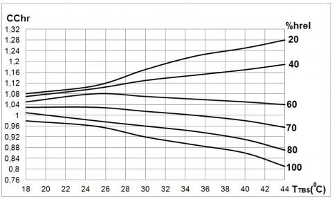
3- Selection of the correction factors due to the wind (Crec) and relative humidity $\text { (CChr) }$ (see Figures 3 and 4).
4- Calculate the real vapor pressure in the turbine outlet as:
$\mathrm{P}_{\mathrm{ST}}=\mathrm{P}_{\mathrm{Back}} \cdot \mathrm{C}_{\mathrm{rec}} \cdot \mathrm{CChr}(\mathrm{kPa})$ (8)
5- Define the steam boiler production $\mathrm{m}_{\mathrm{I}}$, intermediate extraction $\mathrm{m}_{\mathrm{E}}$ and the flow in the turbine exit $\mathrm{m}_{\text {agua }}$.
6-Find the thermodynamic properties (entropy and enthalpy) at inlet $\left(\mathrm{h}_{\mathrm{I}} ; \mathrm{s}_{\mathrm{I}}\right)$, intermediate extraction $\left(\mathrm{h}_{\mathrm{E}} ; \mathrm{s}_{\mathrm{E}}\right)$ and exit of the turbine $\left(\mathrm{h}_{\text {cond }} ; \mathrm{s}_{\text {cond }}\right)$.
7- Define initial thermodynamics parameters of the process, (see Table 3).
Figure 3. Correcting factors due to the wind effect
Figure 4. Correcting factors due to the relative humidity
Table 3. Initial required variables of the combined process
|
Initial required variables |
unit |
|
SPP mill capacity |
t/h |
|
BPP capacity |
MW |
|
Superheated vapor temperature (at steam boiler exit) |
${ }^{\circ} \mathrm{C}$ |
|
Water supply temperature |
${ }^{\circ} \mathrm{C}$ |
|
Vapor temperature in the intermediate extraction |
${ }^{\circ} \mathrm{C}$ |
|
Superheated vapor pressure (at steam boiler exit) |
MPa |
|
Vapor pressure in the intermediate extraction |
MPa |
|
Water supply pressure |
MPa |
|
Vapor flow in the intermediate extraction |
kg/s |
|
Elementary composition of the biomass |
% |
8- Calculate the useful power (in kW) in the turbine installation, using the following equation [9, 10]:
$W_{\text {Elec}}=\left[\begin{array}{c}
m_{\text {agua}} \cdot\left(h_{I}-h_{E}\right)+ \\
+\left(m_{\text {agua}}-m_{E}\right) \cdot\left(h_{E}-h_{\text {cond}}\right)
\end{array}\right] \cdot \eta_{\text {em}} \cdot \eta_{r i}$ (9)
where:
$\eta_{r i}$ and $\eta_{e m}$ are the relative internal and electromechanical performance of the turbine respectively.
9- Find the vapor thermodynamic properties in the turbine outlet, (see Table 4).
Table 4. Thermodynamic properties required, turbine outlet
|
$h_{\text {cond}}$ |
Enthalpy |
$\mathrm{kJ} / \mathrm{kg}$ |
|
$s_{\text {cond}}$ |
Entropy |
$\mathrm{kJ} /\left(\mathrm{kg} \cdot{ }^{\circ} \mathrm{C}\right)$ |
|
$T_{h}$ |
Temperature |
${ }^{\circ} \mathrm{C}$ |
|
$P r_{L}$ |
Prandtl number for single-phase |
- |
|
$\mu_{L}$ |
Liquid dynamic viscosity |
$\mathrm{kg} /(\mathrm{m} \cdot \mathrm{s})$ |
|
$\mu_{V}$ |
Vapor dynamic viscosity |
$\mathrm{kg} /(\mathrm{m} \cdot \mathrm{s})$ |
|
$\rho_{L}$ |
Liquid density |
$\mathrm{kg} / \mathrm{m}^{3}$ |
|
$\rho_{V}$ |
vapor density |
$\mathrm{kg} / \mathrm{m}^{3}$ |
|
$\lambda_{L}$ |
Liquid thermal conductivity |
$\mathrm{W} /\left(\mathrm{m} \cdot{ }^{\circ} \mathrm{C}\right)$ |
|
$C p_{L}$ |
Liquid specific heat |
$\mathrm{kJ} /\left(\mathrm{kg} \cdot{ }^{\circ} \mathrm{C}\right)$ |
10- Establish the arrangements of the tube pack, additionally; the transverse $S_{T}$ and longitudinal pitch $S_{L}$ are required (in m) [11, 12].
11-Establish dimensions of the finned tubes, (all used dimensions are given in m). Fundamentals characteristics are inner and outer diameter of the bare tube ($\mathrm{d}_{\mathrm{i}}$ and $\mathrm{d}_{\mathrm{e}}$ is the inner and outer diameter of the bare tube (without fins), number of fins per linear meter of tube $\mathrm{F}_{\mathrm{a}}$. length of the tube $1$, fins thickness $\mathrm{e}_{\mathrm{a}}$, fins height $\mathrm{h}_{\mathrm{a}}$ and thickness of the tube wall $\mathrm{e}_{\mathrm{T}}$.
12- For a first iteration, select in the Figure 5 an initial value of global heat transfer coefficient K1 [13].
Figure 5. Global heat transfer coefficient for the first iteration
13- For a first iteration, temperature of the condensed outlet can be obtained as:
$\mathrm{T}_{\text {scond }}=\left(\mathrm{T}_{\text {EntVapor }}+\mathrm{T}_{\mathrm{TBS}}\right) / 2\left({ }^{\circ} \mathrm{C}\right)$ (10)
where:
$\mathrm{T}_{\text {EntVapor }}$ is the vapor temperature at ACC inlet, in ℃.
14- By means of the Equation (1) calculate the ITD values.
15- Verify in Figure 2 if ITD obtained value in the step 14 is found in the pink zone, otherwise, an ITD value in the range 22 to 28℃ should be selected.
16-Obtain the LMTD value
$\mathrm{LMTD}=(\mathrm{ITD}-\mathrm{TTD}) / \ln \left(\frac{\mathrm{ITD}}{\mathrm{TTD}}\right)\left({ }^{\circ} \mathrm{C}\right)$ (11)
where:
TTD is the temperature difference on the condensed side, in ℃.
17- Get the enthalpy $\left(\mathrm{h}_{\text {fluid }}\right)$ and entropy $\left(\mathrm{s}_{\text {fluid }}\right)$ of the condensed in the ACC exit.
18- Calculate the rejected heat in the ACC facility.
$Q=m_{\text {agua }} \cdot\left(h_{\text {cond }}-h_{\text {fluid }}\right)(\mathrm{kW})$ (12)
19- Calculate the effective heat transfer surface for a single fin, (m2), as [14]:
$\mathrm{A}_{\mathrm{a}}=\pi \mathrm{e}_{\mathrm{a}}\left(\mathrm{d}_{\mathrm{e}}+2 \mathrm{~h}_{\mathrm{a}}\right)+2 \pi\left[\left(\frac{\mathrm{d}_{\mathrm{e}}}{2}+\mathrm{h}_{\mathrm{a}}\right)^{2}-\left(\frac{\mathrm{d}_{\mathrm{i}}}{2}\right)^{2}\right]$ (13)
20- Determine the number of fins by linear meter of the tube.
$\mathrm{n}_{\mathrm{aT}}=\mathrm{F}_{\mathrm{a}} \cdot \mathrm{l}$ (14)
where: $1$ is the tube length, in m.
21- Determine the heat transfer surface of a single finned tube, by means of the following equation [13]:
$A_{\mathrm{T}}=\pi \mathrm{d}_{\mathrm{e}} \cdot\left(\mathrm{l}-\mathrm{e}_{\mathrm{a}} \mathrm{n}_{\mathrm{aT}}\right)+\mathrm{A}_{\mathrm{a}} \mathrm{n}_{\mathrm{aT}}\left(\mathrm{m}^{2}\right)$ (15)
22- Determine the inner heat transfer surface of the finned tube:
$A_{I}=\pi \cdot l \cdot\left(d_{e}-2 e_{T}\right)\left(m^{2}\right)$ (16)
23- Determine the required heat transfer surface, by means of the following relation:
$\mathrm{F}=\mathrm{Q} /\left(\mathrm{LMTD} \cdot \mathrm{K}_{1}\right)\left(\mathrm{m}^{2}\right)$ (17)
24- Obtain the number of finned tubes of the ACC
$\mathrm{n}_{\mathrm{tubos}}=\mathrm{F} /\left(\mathrm{A}_{\mathrm{T}} \cdot \mathrm{A}_{\mathrm{I}}\right)$ (18)
25- Calculate the liquid and vapor Reynolds number, using the following equations [15]:
$\operatorname{Re}_{\mathrm{L}}=\frac{\mathrm{m}_{\mathrm{agua}} \cdot(1-\mathrm{x}) \cdot \mathrm{d}_{\mathrm{i}}}{\mu_{\mathrm{L}} \cdot 0.785 \cdot \mathrm{d}_{\mathrm{i}}^{2} \cdot \mathrm{n}_{\mathrm{tubos}}}$ (19)
$\operatorname{Re}_{\mathrm{V}}=\frac{\mathrm{m}_{\mathrm{agua}} \cdot \mathrm{x} \cdot \mathrm{d}_{\mathrm{i}}}{\mu_{\mathrm{V}} \cdot 0.785 \cdot \mathrm{d}_{\mathrm{i}}^{2} \cdot \mathrm{n}_{\mathrm{tubos}}}$ (20)
where, $x$ is the thermodynamic vapor quality.
26- Obtain two-phase heat transfer coefficient and drop pressure inside of the tubes using the Camaraza’s methodology [16].
27- Obtain several thermodynamic properties of the air at $\mathrm{T}_{\mathrm{TBS}}$, (see Table 5).
28- Estimate the necessary airflow, as [13]:
$\mathrm{m}_{\text {aire }} \approx \mathrm{Q} /\left[\mathrm{Cp}_{\mathrm{a}}\left(\mathrm{T}_{\mathrm{SACC}}-\mathrm{T}_{\mathrm{TBS}}\right)\right](\mathrm{kg} / \mathrm{s})$ (21)
where: $\mathrm{T}_{\mathrm{SACC}}$ is the air temperature in the exit of the ACC.
29- Calculate the number of fans required.
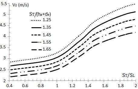
$\mathrm{n}_{\mathrm{vent}} \approx \mathrm{m}_{\mathrm{aire}} /\left(756 \cdot \mathrm{V}_{0}\right)$ (22)
Value of V0 can be obtained in the Figure 6, while $\mathrm{n}_{\mathrm{vent}}$ is rounded to next integer number [13].
Table 5. Thermodynamic properties of the air (at TTBS)
|
$h_{a}$ |
Enthalpy |
$\mathrm{kJ} / \mathrm{kg}$ |
|
$\rho_{a}$ |
Density |
$\mathrm{kg} / \mathrm{m}^{3}$ |
|
$s_{a}$ |
Entropy |
$\mathrm{kJ} /\left(\mathrm{kg} \cdot{ }^{\circ} \mathrm{C}\right)$ |
|
$\lambda_{a}$ |
Thermal conductivity |
$\mathrm{W} /\left(\mathrm{m} \cdot{ }^{\circ} \mathrm{C}\right)$ |
|
$P r_{a}$ |
Prandtl number |
- |
|
$\mu_{a}$ |
Dynamic viscosity |
$\mathrm{kg} /(\mathrm{m} \cdot \mathrm{s})$ |
|
$C p_{a}$ |
Specific heat |
$\mathrm{kJ} /\left(\mathrm{kg} \cdot{ }^{\circ} \mathrm{C}\right)$ |
30- Determinate the maximum velocity of the air in the cross flow through of the minimum flow area (in ACC’s tubes bundle).
Figure 6. Admissible initial velocity of the air in ACC
31- Obtain single-phase heat transfer coefficient and drop pressure in the fins side using the Camaraza’s methodology [13].
32- Define the fouling thermal resistances in both sides of the tubes.
33- Evaluate the assessment performance of a single fin (thermal efficiency), ηA [17].
34- Calculate the efficiency performance of the finned surface [13].
$\eta_{\mathrm{W}}=1-\mathrm{n}_{\mathrm{aT}} \mathrm{A}_{\mathrm{a}}\left(1-\mathrm{n}_{\mathrm{aT}}\right) /\left(\mathrm{A}_{\mathrm{T}} \cdot \mathrm{n}_{\text {tubos }}\right)$ (23)
35- Calculate the global heat transfer (K2).
36- Calculate mean absolute error (MAE) values [18, 19], using coefficients K2 and K1.
$\mathrm{MAE}=100 \cdot\left|\frac{K_{2}-K_{1}}{K_{2}}\right|(\%)$ (24)
If MAE value is lower than 5%, then coefficient K2 are accepted, otherwise, is necessary to repeat the study from the step 11 with the new value of the global heat transfer coefficient K2.
37- Determine the heat transfer surface \mathrm{F}^{\prime} required by the ACC under real conditions of operation [20]:
$\mathrm{F}^{\prime}=\mathrm{Q} /\left(\mathrm{LMTD} \cdot \mathrm{K}_{2}\right)\left(\mathrm{m}^{2}\right)$ (25)
38- Define the expenses required due to ecological trace [17], generated by increase of estimated emissions associated to ACC uses in USD/(GJ·year).
$G_{E m i s}=(6.02-0.434 \cdot B) \cdot A \cdot e^{0.226 \cdot B}$ (26)
where:
e is Euler constant, A and B are constants variables that depend of the volume of emission of greenhouse effect gases. Variables A and B, are computed as [5]:
$A=\ln \left[\left(C O_{2}\right)^{0.1} \cdot S O_{2}\right]^{0.1}+0.252$ (27)
$B=\log \left[\frac{\left(C H_{4} \cdot N O_{X} \cdot(C O)^{0.04}-(S O)^{2}\right)^{2}}{N_{2} O}\right]$ (28)
Volumes of greenhouse effect gases used in Eqns. (27) and (28) are given in Gg.
In the present investigation the methods obtained for the analysis of the heat transfer coefficients are integrated into the developed procedure. The methodology provides a sequence to follow in evaluating the thermal performance of an ACC that operates in conjunction with a TPP.
A case study carried out confirms the coincidence and greater effectiveness of the proposed method, with respect to others existing in the specialized literature.
The developed method allows the analysis of the ACC thermal performance to be carried out in a simple and efficient way, facilitated by the reduction of the uncertainty indices of the methods presented for the determination of the working agent and of the average heat transfer coefficients.
They are considered additional elements that allow estimating the ecological footprint linked to the increase in greenhouse gas emissions generated by the use of ACC.
The authors take this opportunity to warmly thank president of AIGE to give the possibility to publish best papers conference (5th AIGE/IIETA International Conference and XIV AIGE Conference on “Energy Conversion, Management, Recovery, Saving, Storage and Renewable Systems, Ancona, Italy, 2020) in high quality scientific journals.
[1] Gimelli, A., Luongo, A. (2014). Thermodynamic and experimental analysis of a biomass steam power plant: critical issues and their possible solutions with CCGT systems. Energy Procedia, 45: 227-236. https://doi.org/10.1016/j.egypro.2014.01.025
[2] Zaccone, R., Sacile, R., Fossa, M. (2017). Energy modelling and decision support algorithm for the exploitation of biomass resources in industrial districts. International Journal of Heat and Technology, 35(Special Issue 1): S322-S329. https://doi.org/10.18280/ijht.35Sp0144
[3] Sansaniwal, S.K., Pal, K., Rosen, M.A., Tyagi, S.K. (2017). Recent advances in the development of biomass gasification technology: A comprehensive review. Renewable and Sustainable Energy Reviews, 72: 363-384. http://dx.doi.org/10.1016/j.rser.2017.01.038
[4] Sagastume-Gutiérrez, A., Cabello-Eras, J.J., Hens, L., Vandecasteele, C. (2018). Data supporting the assessment of biomass based electricity and reduced GHG emissions in Cuba. Data in Brief, 17: 716-723. https://doi.org/10.1016/j.dib.2018.01.071
[5] Camaraza-Medina, Y. (2020). Current trends in Cuba on the environmental impact and sustainable development. TECNICA ITALIANA-Italian Journal of Engineering Science, 64(1): 103-108. https://doi.org/10.18280/ti-ijes.640116
[6] Huang, X., Chen, L., Kong, Y., Yang, L., Du, X. (2018). Effects of geometric structures of air deflectors on thermo-flow performances of air-cooled condenser. International Journal of Heat and Mass Transfer, 118: 1022-1039. https://doi.org/10.1016/j.ijheatmasstransfer.2017.11.071
[7] Camaraza-Medina, Y., Cruz-Fonticiella, O.M., Garcia-Morales, O.F. (2017). Element for the estimation of thermodynamic properties of cane and forest biomass. Revista Ciencias Técnicas Agropecuarias, 26(4): 76-82.
[8] Camaraza-Medina, Y., Cruz-Fonticiella, O.M., García-Morales, O.F. (2018). Predicción de la presión de salida de una turbina acoplada a un condensador de vapor refrigerado por aire. Centro Azúcar, 45(1): 50-61.
[9] Costa, M., Cirillo, D., Rocco, V., Tuccillo, R., La Villetta, M., Caputo, C., Martoriello, G. (2019). Characterization and optimization of heat recovery in a combined heat and power generation unit. TECNICA ITALIANA-Italian Journal of Engineering Science, 63(2-4): 447-451. https://doi.org/10.18280/ti-ijes.632-448
[10] Gulotta, T.M., Guarino, F., Mistretta, M., Cellura, M., Lorenzini, G. (2018). Introducing exergy analysis in life cycle assessment: A case study. Mathematical Modelling of Engineering Problems, 5(3): 139-145. https://doi.org/10.18280/mmep.050302
[11] Loganathan, P., Dhivya, M. (2018). Thermal and mass diffusive studies on a moving cylinder entrenched in a porous medium, Latin American Applied Research, 48(2): 119-124.
[12] Cano-Moreno, J.D., Cabanellas-Becerra, J.M. (2019). Experimental validation of an escalator simulation model. Latin American Applied Research, 49(3): 187-192.
[13] Camaraza-Medina, Y., Rubio-Gonzales, A.M., Cruz-Fonticiella, O.M., Garcia-Morales, O.F. (2018). Simplified analysis of heat transfer through a finned tube bundle in air-cooled condenser. Mathematical Modelling of Engineering Problems, 5(3): 237-242. https://doi.org/10.18280/mmep.050316
[14] Cucumo, M., Ferraro, V., Galloro, A., Gullo, D., Kaliakatsos, D., Nicoletti, F. (2019). Computational fluid dynamics simulations to evaluate the performance improvement for air-cooler equipped with a water spray system. TECNICA ITALIANA-Italian Journal of Engineering Science, 63(2-4): 158-166. https://doi.org/10.18280/ti-ijes.632-407
[15] Camaraza-Medina, Y., Rubio-Gonzales, A.M., Cruz-Fonticiella, O.M., Garcia-Morales, O.F. (2017). Analysis of pressure influence over heat transfer coefficient on air- cooled condenser. Journal Européen des Systems Automatisés, 50(3): 213-226. http://dx.doi.org/10.3166/jesa.50.213-226
[16] Medina, Y.C., Khandy, N.H., Carlson, K.M., Fonticiella, O.M.C., Morales, O.F.C. (2018). Mathematical modeling of two-phase media heat transfer coefficient in air-cooled condenser systems. International Journal of Heat and Technology, 36(1): 319-324. https://doi.org/10.18280/ijht.360142
[17] Deng, H., Liu, J., Zheng, W. (2019). Analysis and comparison on condensation performance of core tubes in air-cooling condenser. International Journal of Heat and Mass Transfer, 135: 717-731. https://doi.org/10.1016/j.ijheatmasstransfer.2019.02.011
[18] Clymer, J.R. (2017). Mathematics of complex adaptive systems. International Journal of Design & Nature and Ecodynamics, 12(3): 377-384. https://doi.org/10.2495/DNE-V12-N3-377-384
[19] Bian, H., Sun, Z., Cheng, X., Zhang, N., Meng, Z., Ding, M. (2018). CFD evaluations on bundle effects for steam condensation in the presence of air under natural convection conditions. International Communications in Heat and Mass Transfer, 98: 200-208. https://doi.org/10.1016/j.icheatmasstransfer.2018.09.003
[20] Lin, S.C., Tsai, R., Chiu, C.P., Liu, L.K. (2019). A simple approach for system level thermal transient prediction. Thermal Science and Engineering Progress, 9: 177-184. https://doi.org/10.1016/j.tsep.2018.11.013