Changchun Wu | Jianhua Zhu*
© 2026 The authors. This article is published by IIETA and is licensed under the CC BY 4.0 license (http://creativecommons.org/licenses/by/4.0/).
OPEN ACCESS
To address the drawbacks of the conventional hydraulic method in pump efficiency testing, such as the large number of measured parameters and the complexity of the measurement system, this paper derives practical calculation models based on thermodynamic theory, namely the temperature-difference method and the pressure-difference method. The proposed models are validated through engineering case studies; the experimental data are processed by regression analysis using the least-squares method, and the model uncertainty is evaluated in accordance with the International Organization for Standardization (ISO) Guide to the Expression of Uncertainty in Measurement (GUM) standard. The validation results show that the thermodynamic temperature-difference model requires only a few measurement parameters, all of which are easy to obtain, whereas the thermodynamic pressure-difference model—by measuring the differential pressure between the pump inlet and outlet instead of the temperature difference—effectively circumvents the difficulty of measuring minute temperature differences. The thermodynamic pressure-difference method yields reliable test results and fully meets the engineering accuracy requirements for on-site pump efficiency testing, which is of great significance for the accurate measurement of pump efficiency in engineering practice.
thermodynamic temperature-difference method, thermodynamic pressure-difference method, pump efficiency, practical model, validation
As a fluid machine widely used in industrial and agricultural applications, the accurate assessment of pump operating efficiency is important for reducing energy consumption and maintaining efficient system operation. In hydraulic systems, pump pressure, flow rate, and power are closely coupled with operating conditions and constitute fundamental parameters for performance regulation and energy utilization [1]. Accurate determination of pump efficiency is therefore a prerequisite for identifying energy-saving opportunities. At present, there are mainly two methods for testing pump efficiency: the hydraulic method (traditional method) and the thermodynamic method. The main difference between the two methods is that the hydraulic method needs to directly measure the pump flow rate, and then calculate the pump efficiency by using a formula, and the prediction accuracy of the pump efficiency depends on the accuracy of the flow measurement; the thermodynamic method, on the contrary, does not need to directly measure the pump flow rate, and can directly measure the pump efficiency, and then back-calculate the pump flow rate from the shaft power of the pump, thereby obtaining the performance parameters of the pump [2, 3].
The theory of the thermodynamic method was proposed as early as the 1960s [4-6], but constrained by the extreme requirement for the measurement accuracy of temperature difference (millikelvin level), its large-scale engineering application was not gradually carried out until the last ten years or so. Thorne and Neal [7] published a study on the independent evaluation of the thermodynamic method, summarized the practical guidelines and the temperature probe calibration procedures of the direct thermodynamic method, and identified the consistency of the method and the problems to be studied through a series of field comparison tests; the Korean scholar Bae et al. [8] verified the consistency between the thermodynamic method and the classical hydraulic method through precise comparison experiments, confirming the reliability of this method for pump performance assessment; Clifford [9] systematically developed a long-term high-precision differential thermometer set for industrial environments, and achieved a measurement accuracy of 0.29 mK in a throttling calorimeter; Ye et al. [10] proposed an optimized thermodynamic efficiency measurement method adapted to pump-turbines, and completed comparison tests at several pumped storage power stations; Patil [11] applied the thermodynamic theory to other liquid machines; Li et al. [12] introduced entropy production analysis into the loss identification of hydraulic machines for the first time, and subsequent studies have widely applied it to centrifugal pumps, pump-turbines, multi-stage pumps and other equipment. The above studies are mostly limited to specific equipment or laboratory comparisons and therefore provide limited guidance for standardized field assessment across different operating environments. More generally, engineering energy systems require clearly defined and comparable performance indicators if technical performance is to be evaluated consistently across operating conditions [13]. In view of these limitations, it is necessary to establish a thermodynamic-method-based pump efficiency measurement framework that considers both measurement accuracy and engineering practicability, so as to fill the gap between the sophisticated theory and the complex industrial field, and to provide a strong technical guarantee for the energy saving, consumption reduction and safe operation of pump systems.
2.1 Hydraulic method
The hydraulic method is a method in which instruments and meters are used to directly measure the performance parameters of the pump, such as flow rate, head and shaft power, and then these parameters are substituted into Eq. (1) for calculation. It is the standard method for pump performance testing. In order to ensure that accurate results can be obtained under any pump test conditions, a series of industrial standards have been formulated, among which the most important ones include American National Standards Institute (ANSI)/Hydraulic Institute (HI) 14.6-2022, American Society of Mechanical Engineers (ASME) Performance Test Code (PTC) 8.2-2021 and Guo Biao (GB)/Tuijian (T) 20043-2005.
The calculation formula of pump efficiency by the hydraulic method is as follows:
$\eta=\frac{\rho g Q H}{P} \times 100 \%$ (1)
where:
η — efficiency of the pump;
ρ — density of water;
H — head of the pump;
Q — flow rate;
P — shaft power.
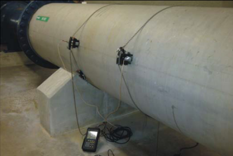
Figure 1. Arrangement of the ultrasonic flowmeter in the hydraulic method
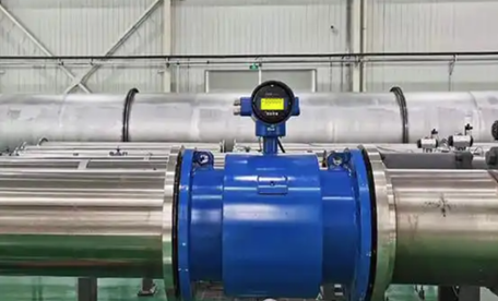
Flow measurement is the most important part in pump efficiency testing. The flow rate is mainly measured by a portable ultrasonic flowmeter (as shown in Figure 1) or an electromagnetic flowmeter installed in the pump station (as shown in Figure 2). Both types of measuring equipment have high requirements on the field test conditions, and factors such as turbulence, air, or bubbles generated by cavitation will significantly affect the accuracy of flow measurement. For flowmeters arranged upstream and downstream, a sufficiently long straight pipe section is required. If the flow measurement equipment is arranged by using the own conditions of a pump station with inlet and outlet flow passages of relatively complex shape, it is difficult to satisfy the conditions of uniform flow or gradually varied flow of the cross-sectional velocity, and thus the test accuracy will be affected [14-16]. In addition, the flowmeters in pump stations are mostly installed on the common pipe or the main pipe, so when other pumps are running at the same time, it is usually impossible to carry out the performance test of a single pump, and it is difficult for most pumps to meet the conditions of high-precision flow measurement [17-19].
Figure 2. Electromagnetic flowmeter on the pump pipeline
2.2 Thermodynamic method
The basic principle of the thermodynamic method is that when the water flows through the pump, friction is generated between the water and the flow passage, and at the same time, friction, eddy and impact are also generated inside the water flow, thus causing mechanical energy loss of the water flow. If the heat exchange between the water flow and the outside and the acoustic energy loss are not taken into account, according to the law of energy conservation and conversion, all this mechanical energy will be converted into heat energy, which raises the temperature of the water flow at the pump outlet. That is, a temperature difference is generated between the inlet and outlet of the pump, and the specific enthalpy of the water flow changes; by measuring and calculating this enthalpy difference, the hydraulic efficiency of the pump can be calculated. Since the thermodynamic method measures the loss item which accounts for a very small proportion of the total energy of the pump, the measurement result has very high accuracy, and it is designated as one of the precision-grade test means in the international standard Deutsches Institut für Normung (DIN) European Norm (EN) International Organization for Standardization (ISO) 5198. However, the measurement of the thermodynamic method requires temperature probes with long-term stability, high precision and high sensitivity, and the application of the thermodynamic method in the field of pump measurement is not yet common.
The efficiency test by the thermodynamic method is simple and easy to carry out, but the accuracy of the temperature difference measurement has a great influence on the pump efficiency. For example, if the efficiency of the pump is 50%, in order to ensure that the efficiency error of the measurement result does not exceed 1%, when the water temperature is 160 ℃ and the pump head is 17.5 MPa, the maximum allowable temperature error is 0.17 ℃; and when the water temperature is 20 ℃ and the pump head is 0.8 MPa, the maximum allowable temperature error is 0.0023 ℃. Therefore, the measurement of the small temperature difference between the inlet and outlet of the pump has, to a certain extent, hindered the popularization and application of the thermodynamic method for measuring pump efficiency, especially the application on pumps at normal temperature and normal pressure [20].
At present, the temperature difference resolution of the laboratory-grade precision temperature difference measuring instrument can reach 0.0001 ℃, which is generally suitable for small temperature difference experiments in the laboratory environment, and the instrument is expensive. Therefore, it is very necessary to study a method that does not need to measure the temperature difference and can still apply the thermodynamic theory to test the pump efficiency.
3.1 Thermodynamic temperature-difference method
According to the thermodynamic steady flow energy equation, the pump efficiency calculation formula (1) can be changed into:
$\eta=\frac{h_{2 s}-h_1}{\left(h_2-h_1\right)+\Delta e^{\prime}}$ (2)
where,
η — efficiency of the pump;
h₂ₛ — specific enthalpy at the pump outlet under the ideal state (isentropic process);
h₁ — specific enthalpy at the pump inlet in the actual non-isentropic compression process;
h₂ — specific enthalpy at the pump outlet in the actual non-isentropic compression process;
$\Delta e^{\prime}$ — the part of the heat energy converted from various losses that is not absorbed by the liquid.
According to the thermodynamic theory, the calculation formula of the enthalpy change under the ideal state (isentropic process) is as shown in Eq. (3), and the calculation formula of the enthalpy change under the actual non-isentropic state is as shown in Eq. (4).
$h_{2 s}-h_1=\bar{v}\left(p_2-p_1\right)$ (3)
where,
$\bar{v}$ — mean specific volume of water;
$p_2-p_1$ — pressure difference between the inlet and outlet of the pump.
$h_2-h_1=\bar{a}\left(p_2-p_1\right)+\bar{C}_p\left(T_2-T_1\right)$ (4)
where,
$\bar{a}$ — coefficient of compressibility of water, which is called the isentropic factor in the international standard;
$\bar{C}_p$ — mean specific heat capacity of water;
$T_2-T_1$ — temperature difference between the inlet and outlet of the pump.
Substituting Eqs. (3) and (4) into Eq. (2), the basic mathematical model for testing the pump efficiency by the thermodynamic method can be obtained as follows:
$\eta=\frac{\bar{v}\left(p_2-p_1\right)}{\bar{a}\left(p_2-p_1\right)+\bar{C}_p\left(T_2-T_1\right)+\Delta e^{\prime}}$ (5)
According to different objects and needs, different simplifications and calculations can be carried out on Eq. (5). Dividing the numerator and the denominator of Eq. (5) by $\bar{v}\left(p_2-p_1\right)$ at the same time, Eq. (6) is obtained.
$\eta=\frac{1}{\frac{\bar{a}}{\bar{v}}+\frac{\bar{C}_p\left(T_2-T_1\right)}{\bar{v}\left(p_2-p_1\right)}+\frac{\Delta e^{\prime}}{\bar{v}\left(p_2-p_1\right)}}$ (6)
Because the pump head $H=\frac{\bar{v}\left(p_2-p_1\right)}{g}$, Eq. (6) can be changed into:
$\eta=\frac{1}{\frac{\bar{a}}{\bar{v}}+\frac{\bar{C}_p\left(T_2-T_1\right)+\Delta e^{\prime}}{g H}}$ (7)
Under different pressures and different temperatures, the pump efficiency can all be calculated according to the above equation. Taking the case of 1 standard atmospheric pressure and a water temperature of 20 °C as an example, it is found from the tables that: $\bar{C}_p=4186 \mathrm{~J} /(\mathrm{kg} \cdot \mathrm{K})$, $\bar{v}=0.001002 \mathrm{~m}^3 / \mathrm{kg}$, $\bar{a}=9.39 \times 10^{-4} \mathrm{~m}^3 / \mathrm{kg}$, $g=9.81 \mathrm{~m} / \mathrm{s}^2$. Substituting these into Eq. (7) gives:
$\eta=\frac{1}{0.937+\frac{426.7 \Delta T}{H}+\frac{\Delta e^{\prime}}{\mathrm{g} H}}$ (8)
where,
$\Delta T$ — temperature difference between the outlet and inlet of the pump;
H — head of the pump.
$\Delta e^{\prime}$ is mainly the bearing and shaft seal friction losses and the heat dissipation loss of the pump casing, and the proportion of the losses is usually less than $1 \%$. In general engineering applications, item $\Delta e^{\prime}$ can be neglected, and then the above equation can be simplified as:
$\eta=\frac{1}{0.937+\frac{426.7 \Delta T}{H}}$ (9)
3.2 Thermodynamic pressure-difference method
In order to solve the problem of the difficult measurement of the small temperature difference between the inlet and outlet of the pump, some researchers have adopted the partial expansion method and the zero temperature-difference method [20]. These two methods do not directly measure the small temperature difference between the inlet and outlet of the pump, but use the pressure loss caused by the pressure reducing device installed in the pressure measuring pipeline, which corresponds to the temperature rise, for measurement. Specifically, a sampling water flow is extracted at the pump inlet, and an expansion valve is set between the sampling pipeline and the remaining measuring components, so that the temperature of the water flow rises to the pump outlet temperature after passing through the expansion valve. In this way, in the denominator of the pump efficiency calculation Eq. (5), item $\bar{C}_p\left(T_2-T_1\right)$ becomes zero, and the pressure at this time $p_{11}$ is measured by a pressure sensor with sufficient accuracy, and item $\bar{a}\left(p_2-p_1\right)$ in the denominator of Eq. (5) becomes $\bar{a}\left(p_2-p_{11}\right)$, so that the efficiency value can be determined, and its expression is as follows:
$\eta=\frac{\bar{v}\left(p_2-p_1\right)}{\bar{a}\left(p_2-p_{11}\right)+\Delta e^{\prime}}$ (10)
The partial expansion method and the zero temperature-difference method can carry out the measurement and achieve a very high accuracy under the condition that the temperature difference between the inlet and outlet of the pump is very small, but the actual measurement process is relatively complicated, and the measuring pipeline cannot work in an environment lower than the atmospheric pressure, so there are few engineering applications. However, according to the design concept of the zero temperature-difference method, the temperature difference $\Delta T$ in Eq. (8) can be expressed in the form of pressure and pressure difference, namely:
$\eta=\frac{1}{0.937+\frac{426.7}{H} \mu\left(\frac{p_1}{p_a}\right)^n\left(\frac{\Delta p}{p_2}\right)^m}$ (11)
where,
$p_1$ — absolute pressure at the inlet of the pump;
$p_2$ — absolute pressure at the outlet of the pump;
$\Delta p$ — pressure difference between the outlet and inlet of the pump;
$p_a$ — atmospheric pressure;
$\mu$ — coefficient, taken as 1.01;
m, n — exponents.
According to Karassik et al. [21], m = 0.75-1, n = 1.75-2.
Using pressure measurement instead of temperature difference measurement not only avoids the technical and cost problems of small temperature difference measurement, but also has a small time-lag coefficient and a fast response of pressure measurement, which is beneficial to the on-line testing of pump efficiency. The thermodynamic pressure-difference method test system for pump efficiency is simpler, and the test process is more convenient, and it is a simple and practical water efficiency test model.
4.1 Main technical indicators of the test equipment
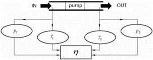
In order to verify the scientificity and engineering applicability of the efficiency calculation model of the thermodynamic pressure-difference method, two clean water centrifugal pumps with different power levels were selected for performance tests under variable operating conditions. The measurement schematic diagram is shown in Figure 3.
(1) Pressure test equipment
The inlet and outlet pressure test of the pump adopts the Rosemount 3051S pressure transmitter, and the main technical parameters are as follows:
Stability: ± 0.2% of the upper range limit value (10 years)
Reference accuracy: ± 0.025% of the span
Range ratio: 200:1
Measuring range: differential pressure measurement 2000 psi (137.89 bar), gauge pressure measurement 2000 psig (137.89 bar), absolute pressure measurement 4000 psia (275.79 bar)
(2) Temperature test equipment
The inlet and outlet pressure test of the pump adopts the Anton-Paar MKT-50 precision temperature measuring instrument, and the main technical parameters are as follows:
Measuring range: temperature −260 ℃ to +962 ℃
Resolution: 0.0001 ℃
Measurement uncertainty: temperature < 1 mK (Pt 100)
Temperature sensor: Pt 100 or Pt 25.5
Measuring time: 1.44 s (two channels)
Ambient temperature for use: 0 ℃ to 35 ℃ (the recommended temperature for the highest accuracy is 20 ℃ to 25 ℃).
Figure 3. Schematic diagram of the pump efficiency test
4.2 Case 1: Small centrifugal pump
The test was carried out under the environment of a local atmospheric pressure of 101.2 kPa and a temperature of 20 ℃, and the performance test was carried out on an IS80-50-315 clean water centrifugal pump. Under the design condition, the flow rate Q of this pump is 50 m³/h, the head H is 125 m, the rated rotational speed is 2900 r/min, and the shaft power P is 31.5 kW.
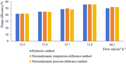
In the test, the inlet and outlet water temperature difference, pressure and shaft power parameters at 5 different flow rates were measured respectively, and the original data are shown in Table 1.
Table 1. Original test data of the IS80-50-315 clean water centrifugal pump
|
Parameter Name / Unit |
Flow Rate/m³·h-1 |
||||
|
23.5 |
27.9 |
35.7 |
51.8 |
60.1 |
|
|
Inlet and outlet water temperature difference/℃ |
0.452 |
0.398 |
0.322 |
0.248 |
0.235 |
|
Inlet vacuum/kPa |
36.1 |
39.8 |
45.9 |
54.9 |
56.3 |
|
Inlet absolute pressure/kPa |
65.1 |
61.4 |
55.3 |
46.3 |
44.9 |
|
Outlet gauge pressure/kPa |
1301.2 |
1252.3 |
1183.4 |
1162.1 |
1002.3 |
|
Outlet absolute pressure/kPa |
1402.4 |
1353.5 |
1284.6 |
1263.3 |
1103.5 |
|
Inlet and outlet absolute pressure difference/kPa |
1337.3 |
1292.1 |
1229.3 |
1217.0 |
1058.6 |
|
Head/m |
132.6 |
131.9 |
128.3 |
125.2 |
101.6 |
|
Shaft power/kW |
20.4 |
22.3 |
25.6 |
31.6 |
33.2 |
Table 2. Calculation results of the pump efficiency of the IS80-50-315 clean water centrifugal pump
|
Calculation Method |
Flow Rate/m³·h-1 |
Remark |
||||
|
23.5 |
27.9 |
35.7 |
51.8 |
60.1 |
||
|
Efficiency by the hydraulic method/% |
41.58 |
44.92 |
48.71 |
55.87 |
50.10 |
Calculated by Eq. (1) |
|
Efficiency by the thermodynamic temperature-difference method/% |
41.81 |
44.95 |
49.80 |
56.11 |
51.98 |
Calculated by Eq. (9) |
|
Efficiency by the thermodynamic pressure-difference method/% |
41.91 |
44.38 |
48.41 |
55.90 |
51.85 |
Calculated by Eq. (11) |
Figure 4. Pump efficiency values of the IS80-50-315 clean water centrifugal pump calculated by the three methods
Table 3. Original test data of the IS125-100-315 clean water centrifugal pump
|
Parameter Name / Unit |
Flow Rate/m³·h-1 |
||||
|
82.3 |
119.2 |
159.1 |
199.8 |
224.0 |
|
|
Inlet and outlet water temperature difference/℃ |
0.431 |
0.278 |
0.189 |
0.124 |
0.136 |
|
Inlet vacuum/kPa |
38.9 |
50.8 |
60.8 |
70.4 |
68.0 |
|
Inlet absolute pressure/kPa |
62.3 |
50.4 |
40.4 |
30.8 |
33.2 |
|
Outlet gauge pressure/kPa |
1283.1 |
1269.3 |
1194.6 |
1159.8 |
1010.7 |
|
Outlet absolute pressure/kPa |
1384.3 |
1370.5 |
1295.8 |
1261.0 |
1111.9 |
|
Inlet and outlet absolute pressure difference/kPa |
1322.0 |
1320.1 |
1255.4 |
1230.2 |
1078.7 |
|
Head/m |
134.9 |
134.7 |
128.1 |
121.5 |
106.3 |
|
Shaft power/kW |
70.1 |
81.2 |
88.7 |
93.7 |
97.2 |
Table 4. Calculation results of the pump efficiency of the IS125-100-315 clean water centrifugal pump
|
Calculation Method |
Flow Rate/m³·h-1 |
Remark |
||||
|
82.3 |
119.2 |
159.1 |
199.8 |
224.0 |
||
|
Efficiency by the hydraulic method/% |
43.11 |
53.83 |
62.55 |
70.53 |
66.69 |
Calculated by Eq. (1) |
|
Efficiency by the thermodynamic temperature-difference method/% |
43.47 |
55.02 |
63.83 |
72.86 |
67.43 |
Calculated by Eq. (9) |
|
Efficiency by the thermodynamic pressure-difference method/% |
44.29 |
53.89 |
62.66 |
72.93 |
66.64 |
Calculated by Eq. (11) |
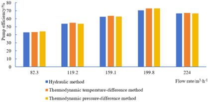
Figure 5. Pump efficiency values of the IS125-100-315 clean water centrifugal pump calculated by the three methods
4.3 Case 2: Large centrifugal pump
In order to further verify the generalization ability of the model on high-power pumps, under the same environmental conditions as those in Case 1, a performance test was carried out on an IS125-100-315 clean water centrifugal pump. Under the design condition of this pump, the flow rate Q = 200 m³/h, the head H = 125 m, the rated rotational speed is 2900 r/min, and the shaft power P = 90.8 kW. In the test, the test data at 5 different flow rates were measured, and the original data are shown in Table 3.
Similarly, taking m = 0.75 and n = 1.75, the efficiency by the pressure-difference method under each operating condition of Case 2 was calculated by using Eq. (11), and the results are shown in Table 4. The data results in Table 4 are plotted in Figure 5.
4.4 Regression analysis of the model parameters based on the least-squares method
In order to further verify the rationality of the values of the empirical exponents m and n in Eq. (11), in this section, based on a total of 10 sets of test data from the two engineering cases, the least-squares method is used to carry out the parameter identification of the model.
(1) Goodness of fit
Eq. (11) is a nonlinear function. In order to facilitate the solution by the least-squares method, the natural logarithm is taken on both sides of it for linearization:
$\begin{aligned} \ln \left(\frac{1}{\eta}-0.937\right) & =\ln \left(\frac{426.7 \mu}{H}\right) +n \ln \left(\frac{p_1}{p_a}\right)+m \ln \left(\frac{\Delta p}{p_2}\right)\end{aligned}$ (12)
Let $Y=\ln \left(\frac{1}{\eta}-0.937\right)-\ln \left(\frac{426.7 \mu}{H}\right)$, the independent variables $X_1=\ln \left(\frac{p_1}{p_a}\right)$, $X_2=\ln \left(\frac{\Delta p}{p_2}\right)$, then Eq. (12) can be simplified as:
$Y=n X_1+m X_2+\varepsilon$ (13)
where,
$\varepsilon$ — random error.
Taking the efficiency by the thermodynamic temperaturedifference method as the true efficiency and substituting it into the calculation, in the calculation, atmospheric pressure $p_a$ is taken as 101.2 kPa and coefficient $\mu$ is taken as 1.01. It can be obtained by calculation that: m = 0.772, n = 1.768, the regression sum of squares (SSR) is 2.4738, the residual sum of squares (SSE) is 0.0471 , the total sum of squares (SST) is 2.5209, and the goodness of fit $R^2$ is 0.981 , which indicates that the goodness of fit is extremely high.
(2) Residual distribution diagnosis
Substituting m = 0.772 and n = 1.768 obtained by the regression into Eq. (11), the predicted efficiencies of the 10 operating condition points of the two cases were calculated, and the residuals were calculated, and the results are shown in Table 5.
From the residual distribution, the absolute values of the residuals of the 10 operating condition points are all less than 0.55%, and the signs of the residuals show a random distribution characteristic of "alternating positive and negative", and no obvious U-shaped or monotonic trend appears, which indicates that the functional structure of Eq. (11) can correctly describe the mapping relationship between the thermodynamic pressure difference inside the pump and the efficiency, and the regression model has no systematic deviation.
Table 5. Predicted efficiency and residuals of the regression model
|
Case |
Flow Rate/m³·h-1 |
Efficiency by the Temperature-Difference Method/% |
Efficiency by the Regression Model/% |
Residual/% |
|
Case 1 |
23.5 |
41.81 |
41.75 |
0.06 |
|
27.9 |
44.95 |
44.62 |
0.33 |
|
|
35.7 |
49.80 |
49.28 |
0.52 |
|
|
51.8 |
56.11 |
55.74 |
0.37 |
|
|
60.1 |
51.98 |
51.76 |
0.22 |
|
|
Case 2 |
82.3 |
43.47 |
43.21 |
0.26 |
|
119.2 |
55.02 |
55.31 |
-0.29 |
|
|
159.1 |
63.83 |
64.15 |
-0.32 |
|
|
199.8 |
72.86 |
72.71 |
0.15 |
|
|
224.0 |
67.43 |
67.62 |
-0.19 |
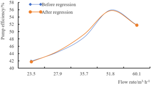
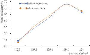
The relationship between the pump flow rate and the efficiency before and after the regression is shown in Figure 6 and Figure 7.
Figure 6. Flow rate–efficiency curve of the IS80-50-315 clean water centrifugal pump
Figure 7. Flow rate–efficiency curve of the IS125-100-315 clean water centrifugal pump
(3) Adoption of the engineering recommended values
The exponents n = 1.768 and m = 0.772 obtained by the regression are within the lower limit of the recommended range for small pumps given in References [21, 22] (m = 0.75–1, n = 1.75–2), which confirms the theoretical rationality of this empirical formula from the data level.
Considering that there is a natural correlation between $\Delta p$ and $p_2$ in Eq. (11) $\left(\Delta p / p_2 \approx 0.95\right)$, and the variance of $X_2$ is small, the stability of the regression coefficient $m$ is sensitive to the sample size. In order to facilitate the practical engineering application and ensure the generalization ability of the model, this study finally adopts the integer values $m=$ 0.75 and $n=1.75$ recommended in the literature as the engineering parameters of Eq. (11). The verification shows that the efficiency deviation between the calculated results using the recommended values and the regression values does not exceed $0.3 \%$, which fully meets the requirements of engineering measurement accuracy.
In order to comprehensively evaluate the reliability of the thermodynamic pressure-difference method (Eq. (11)) in practical engineering application, based on the internationally used ISO Guide to the Expression of Uncertainty in Measurement (GUM) framework, a quantitative analysis is carried out on the uncertainty of the final pump efficiency caused by the measurement uncertainty of the core measurement parameters in the model (the inlet absolute pressure $p_1$, the outlet absolute pressure $p_2$ and the atmospheric pressure $p_a$).
5.1 Measurement model and uncertainty propagation law
According to the uncertainty propagation law of ISO GUM, when the input quantities are independent of each other, the combined standard uncertainty $u_c(\eta)$ of input $\eta$ is:
$\begin{aligned} & u_c(\eta)=\sqrt{\left(\frac{\partial \eta}{\partial p_1} u\left(p_1\right)\right)^2+\left(\frac{\partial \eta}{\partial p_2} u\left(p_2\right)\right)^2+\left(\frac{\partial \eta}{\partial p_a} u\left(p_a\right)\right)^2}\end{aligned}$ (14)
Let the sensitivity factor $K=1-0.937 \eta$, and the sensitivity coefficients of the input quantities are derived:
(1) Sensitivity coefficient of the inlet absolute pressure $p_1$:
$c_{p 1}=-\eta K\left(\frac{n}{p_1}-\frac{m}{p_2-p_1}\right)$ (15)
(2) Sensitivity coefficient of the outlet absolute pressure $p_2$:
$c_{p 2}=-\eta K m\left(\frac{1}{p_2-p_1}-\frac{1}{p_2}\right)$ (16)
(3) Sensitivity coefficient of the atmospheric pressure $p_a$:
$c_{p a}=\eta K n \frac{1}{p_a}$ (17)
5.2 Calculation of a typical operating condition example
The test data of Case 1 at the optimum operating point (flow rate Q = 51.8 m³/h) are selected for substitution and checking calculation.
Operating condition parameters: the pump efficiency by the thermodynamic temperature-difference method $\eta=56.11 \%$, the pump head $\mathrm{H}=125.2 \mathrm{~m}$, the pump inlet absolute pressure $p_1=46.3 \mathrm{kPa}$, the pump outlet absolute pressure $p_2=1263.3$ kPa , and the atmospheric pressure $p_a=101.2 \mathrm{kPa}$.
Model parameters: m = 0.75, n = 1.75, and the sensitivity factor is calculated as K = 0.474.
Substituting the above data into the uncertainty propagation formula, the calculation results are shown in Table 6.
Table 6. Summary table of the uncertainty components of the pump efficiency measurement
|
Uncertainty Source |
Sensitivity Coefficient |
Efficiency Uncertainty Component/% |
Variance Contribution Rate/% |
|
Inlet absolute pressure $p_1$ |
-9.89 × 10⁻³ |
0.914 |
99.79 |
|
Outlet absolute pressure $p_2$ |
-5.98 × 10⁻⁶ |
0.00055 |
<0.01 |
|
Atmospheric pressure $p_a$ |
-4.6 × 10⁻³ |
0.0267 |
0.2 |
|
Combined standard uncertainty |
- |
0.915 |
100 |
Taking the coverage factor k = 2 (corresponding to a confidence probability of about 95%), it can be obtained that the expanded uncertainty is 1.83%.
From the analysis of the above calculation results, it can be known that:
(1) The inlet pressure $p_1$ is the absolute dominant factor of the measurement uncertainty. It can be seen from the variance contribution rate that the uncertainty of $p_1$ contributes 99.79% of the total variance. It is suggested that in the measurement by the pressure-difference method, a high-precision (>0.05% FS) pressure sensor must be used for the inlet absolute pressure $p_1$, and this is the core way to improve the accuracy of the efficiency measurement.
(2) The uncertainty of the outlet pressure $p_2$ can be neglected.
(3) The influence of the atmospheric pressure $p_a$ is at a relatively low level. Since the reference value of $p_a$ is large, its variance contribution is only 0.20%, and the use of a conventional digital barometer can meet the engineering requirements.
(4) Mutual confirmation with the results of the residual analysis.
The ISO GUM analysis shows that, under the instrument accuracy of 0.1% FS, the theoretical combined standard uncertainty of the model is about 0.915%. Combined with the residual diagnosis results in Table 5, it can be seen that the residuals are completely within the coverage range of the theoretical uncertainty (k = 1), and are mainly caused by the small measurement error of the inlet pressure. This verifies, from the metrological point of view, the reliability and the accuracy margin of Eq. (11) as an engineering application model, and it fully meets the engineering accuracy requirements of the on-site pump efficiency test.
It should be noted that in the model of this paper, both the density and the specific heat capacity are taken as the constants corresponding to 20 ℃. Within the range of 20 ± 0.23 ℃, the change rate of the density of water is about 2.3 × 10⁻⁴ kg·m⁻³·℃⁻¹, and the change rate of the specific heat capacity is about 1 × 10⁻³ kJ·kg⁻¹·℃⁻¹. The relative error of the density introduced thereby does not exceed 5 × 10⁻⁵, and the relative error of the specific heat capacity does not exceed 2 × 10⁻⁴. Through error propagation, the combined influence of the two on the heat exchange quantity obtained by the pressure-difference method does not exceed 0.07%, which is smaller than the relative error of the temperature difference corresponding to the calibration uncertainty of the temperature sensor itself. Therefore, under the operating conditions studied in this paper, neglecting the continuous correction of the physical properties with temperature will not have a substantial influence on the main conclusions.
(1) The measurement of the pump efficiency by the thermodynamic temperature-difference method has few measurement parameters, a simple system, convenient operation and easy measurement, but according to the model checking calculation data, a relatively low pump head will produce a relatively large error, and it is recommended to be used for pumps with a head greater than 20 m.
(2) The thermodynamic pressure-difference method uses the measurement of the pressure difference between the inlet and outlet of the pump instead of the temperature difference measurement, which effectively circumvents the difficult problem of small temperature difference measurement, is basically not limited by the accuracy of the temperature measuring equipment, and is of great significance for the accurate testing of the pump efficiency in engineering practice.
(3) The practice has proved that the calculation model of the thermodynamic pressure-difference method for the pump efficiency fully meets the engineering accuracy requirements of the on-site pump efficiency test, and it is a practical method for promoting the application of the thermodynamic method in the pump efficiency test.
This paper was supported by the Scientific Research Project of Anhui Provincial Department of Education (Grant No.: 2024AH050580).
[1] Jovanović, V., Janošević, D. (2023). Analysis and regulation of mechatronic systems in advanced mobile machines. Journal of Engineering Management and Systems Engineering, 2(3): 140-149. https://doi.org/10.56578/jemse020301
[2] Gülich, J.F. (2020). Centrifugal Pumps (3rd ed.). Cham: Springer.
[3] Ge, M., Petkovšek, M., Zhang, G., Jacobs, D., Coutier-Delgosha, O. (2021). Cavitation dynamics and thermodynamic effects at elevated temperatures in a small Venturi channel. International Journal of Heat and Mass Transfer, 170: 120970. https://doi.org/10.1016/j.ijheatmasstransfer.2021.120970
[4] Whillier, A. (1967). Pump efficiency determination from temperature measurements. South African Mechanical Engineer, 10: 153-160.
[5] Nihill, J., Date, A., Velardo, J., Jadkar, S. (2018). Experimental investigation of the thermal power pump cycle–Proof of concept. Applied Thermal Engineering, 134: 182-193. https://doi.org/10.1016/j.applthermaleng.2018.01.106
[6] Sitranon, J., Lertsatitthanakorn, C., Namprakai, P., Prathinthong, N., Suparos, T., Roonprasang, N. (2015). Parametric consideration of a thermal water pump and application for agriculture. Journal of Solar Energy Engineering, 137(3): 031006. https://doi.org/10.1115/1.4029108
[7] Thorne, E.W., Neal, A.N. (2000). Pump efficiency testing by the thermodynamic method—An independent view. Proceedings of the Institution of Mechanical Engineers, Part A: Journal of Power and Energy, 214(3): 255-268. https://doi.org/10.1243/0957650001538344
[8] Bae, C.O., Vuong, D.P., Lee, H.I. (2012). A study on the pump efficiency measurement using the thermodynamic method. Journal of the Korean Society of Marine Environment & Safety, 18(3): 267-272.
[9] Clifford, T. (2022). Towards long term, high accuracy difference thermometer sets for the purpose of measuring the efficiency of turbomachinery (Doctoral dissertation). University of Exeter.
[10] Ye, Z., Chen, D., Zhang, Z., Lin, Z. (2025). Efficiency measurement for pump-turbine by thermodynamic test method. Journal of Physics: Conference Series, 3150(1): 012123. https://doi.org/10.1088/1742-6596/3150/1/012123
[11] Patil, S. (2010). Efficiency measurement of hydraulic machines by thermodynamic method. International Journal of Engineering Research and Applications, 2(4): 1542-1547.
[12] Li, Q., Chen, J., Lin, X., Yi, C., Hu, Y. (2026). Entropy-based analysis of near-wall flow and energy dissipation mechanisms in a centrifugal pump with biomimetic microstructured blades. Flow Measurement and Instrumentation, 109: 103212. https://doi.org/10.1016/j.flowmeasinst.2026.103212
[13] Shafie, S.M., Rhofita, E.I. (2026). Performance indicators for energy storage in Malaysia’s energy transition: A systematic review and sustainable supply chain management framework. Journal of Engineering Management and Systems Engineering, 5(3): 354-376. https://doi.org/10.56578/jemse050305
[14] Stoffel, B., Willm, G. (2004). Thermodynamic efficiency measurement on centrifugal pumps: Comparison of different measurement methods. Proceedings of the Institution of Mechanical Engineers, Part A: Journal of Power and Energy, 218(4): 271-278.
[15] Tang, Q.H., Yu, A., Zheng, Y., et al. (2020). Influence of thermodynamic effects on cloud cavitation dynamics characteristics around 3D hydrofoil. Journal of Drainage and Irrigation Machinery Engineering, 38(6): 553-559.
[16] Li, D., Miao, B., Li, Y., Gong, R., Wang, H. (2021). Numerical study of the hydrofoil cavitation flow with thermodynamic effects. Renewable Energy, 169: 894-904. https://doi.org/10.1016/j.renene.2021.01.073
[17] Li, H., Chen, Y., Bai, L., Shi, W., Zhou, L. (2024). Assessing energy loss and entropy production in a centrifugal pump with various impeller blade trailing edges. Journal of Applied Fluid Mechanics, 18(2): 518-534. https://doi.org/10.47176/jafm.18.2.2488
[18] Willm, G., Stoffel, B. (2004). Thermodynamic efficiency measurement on centrifugal pumps: Influence of heat transfer on measurement uncertainty. Proceedings of the Institution of Mechanical Engineers, Part A: Journal of Power and Energy, 218(4): 261-270.
[19] Papaf, R.D. (2013). Canada takes a lead in benchmarking pump energy efficiency. Water, 21: 30-33.
[20] Rossetti, A., Ferrari, L. (1982). Thermodynamic measurement of pump efficiency: Experimental results on a centrifugal pump. La Termotecnica, 36(10): 55-62.
[21] Karassik, I.J., Messina, J.P., Cooper, P., et al. (2008). Pump Handbook (4th ed.). New York: McGraw-Hill.