Sajjad Tariq A. Shafi | Mohammed K. Al-Saadi | Ameer Abed Jaddoa*
© 2026 The authors. This article is published by IIETA and is licensed under the CC BY 4.0 license (http://creativecommons.org/licenses/by/4.0/).
OPEN ACCESS
The demand for electric and heat energy has risen significantly in recent years. Consequently, renewable energy (RE) resources in both systems are increasingly regarded by researchers as vital solutions to rising loads. Optimal microgrid (MG) planning for combined electric and heat loads enhances operational efficiency and reduces emissions. This paper presents an optimal operation framework for a combined heat and power (CHP) smart distribution grid, incorporating RE and solar air heaters (SAH). Initially, an SAH is designed and implemented, followed by various approaches and experiments aimed at enhancing its performance. The integration of SAHs with the proposed system facilitates an analysis of their effects on system operation. The optimization problem is framed as a unit commitment multi-objective mixed nonlinear program (UCMOMNLP), wherein greenhouse gas emissions are monetized to streamline the multi-objective optimization into a singular objective. Furthermore, numerous realistic constraints are integrated to align the approach with practical scenarios. Results indicate a 12.58% reduction in total cost with SAH utilization.
combined heat and power, emission cost, microgrid, mixed integer non-linear programming, multi-objective optimization, solar air heater, unit commitment
With the development of civilization, the demand for energy increases sharply. However, 81% of the energy is supplied by generation sources driven by fossil fuels. These energy resources emit greenhouse gases, which damage the environment and cause global warming. It is important to reach the carbonian neutrality by 2050 in line with the Paris Protocol to limit the emission of greenhouse gases [1]. Buildings are one of the most energy-consuming sectors, as they consume about 40% of the total global energy consumption and contribute about 28% of emissions. Therefore, it is necessary to shift towards the use of renewable energy (RE) sources as an alternative, environmentally friendly energy source to confront climate change and the sustainability of available energy resources [2-7].
In traditional energy grids, the transmission of energy from power plants to the far loads increases energy losses. The wide integration of RE with the power grids increases the complexity of the operation of the grid [5]. Recently, energy sources are installed close to the end user consumer to minimize the losses and energy waste. Microgrid (MG) is the connection of these energy resources close to the end users [8-14]. MG is a low-voltage distribution network that has independent control and can be operated either in separate (island) mode or connected mode with the grid. The MG has many energy sources, including distributed generation (DG), microturbine (MT), and RE, and has energy storage systems (ESSs) in order to achieve optimal use of resources to ensure supplying the load [15]. The MG system is flexible and efficient as it is able to manage energy production according to demand response, unlike conventional systems that may waste half of the energy produced [5]. Exacerbating the problem is the integration of RE sources with the grid due to the stochastic nature of RE and the uncertainty of load demand. Additionally, peak times for energy production from renewable sources occur during periods of low load demand, that affecting the stability of the grid [16]. Currently, the MG supplies both electric and heat loads simultaneously in one entire framework, which is called a combined heat and power microgrid (CHP-MG). contain solar collectors as solar air heaters (SAH) that provide heat to achieve the maximum benefit from the energy coming from the sun [17]. Additionally, the wasted heat which was released when producing electricity can be recovered and reused in utilized benefit heat applications within the system of heating and other applications [18-23].
In order to minimize operation costs and emissions of green gas at produce power while enhancing the reliability and stability of grids, the literature discusses various methods to improve the operation of CHP-MG, multi optimizations approaches used as unit commitment (UC), Heuristic algorithm, genetic algorithm (GA), particle swarm optimization (PSO), and other approaches [24].
Pashaei-Didani et al. [25] modeled an MG system with base CHP, power sources, FC, and storage systems connected to the grid, to minimize cost and emissions by scheduling a demand response program (DRP) with multi-objective Pareto solutions by using the compromising programming approach; then, the optimal solution is chosen by implementing the fuzzy satisfying approach. This approach reduced the set of effective solutions. The use of DRP reduced cost and emissions by 2.8% and 126 kg. In the previous study, distributed energy resources (DERs) and ESSs were used to share the required electricity demand from controllable and uncontrollable loads in short-term scheduling of thermal and electrical grids [26]. As for the authors of study [16], they integrated solar and wind energy sources while prioritizing renewable energy; the Particle Swarm Optimization (PSO) algorithm was used to improve consumption, saving 283.91 MW. According to the demand response with the environmental constraint method, the fuzzy satisfaction approach was used to choose the best compromise solution that was the least cost and the effect of the time DRP on MG in scheduling time demand response, which cost $3652 and emitted 53150.16 tons/day. In the same construction system, previous literature [27] used the multi-objective bacterial colony chemotaxis (MOBCC) algorithm with the Order of Preference by Similarity to the Ideal Solution (TOPSIS) method to choose the final decision solution [28]. Use District Heating Network (DHN) with CHP and buffer tank storage for extra flexibility, as it is able to adjust its electrical power production very quickly, while meeting the heat demand.
In this study, an energy management system of a CHP-MG with integration of renewable sources and SAHs to meet electrical and thermal loads is proposed. The CHP grid contains fuel cells (FCs), MTs, diesel generators (DG), wind turbine (WT), photovoltaic panels (PV), and electrical ESS. Meanwhile, the heat demand is met from the MTs heat recovery (HR) system, gas boiler, the electric heater (EH), and the heat storage system (HSS). Besides, the SAH, which was practically implemented in a previous study [29] and tested, has different designs to determine which design has the lowest operational cost of the system, supplies heat loads. The system was also connected to the public utility grid, where the system can trade heat and electric energy with the utility grid. The proposed problem is formulated as Unit commitment Mixed-Integer Non-Linear Programming (UCMINLP) hourly, employed GAMS software to solve the optimization, also modeling the interaction between the electrical and heat systems, Consider the operational cost of the electrical and heat systems of the network, and the objectives function of multi -objective converted to improving the single objective by considering the costs of the CO2, SO2, NOx and particulate matter (PM) to the monetary concept.
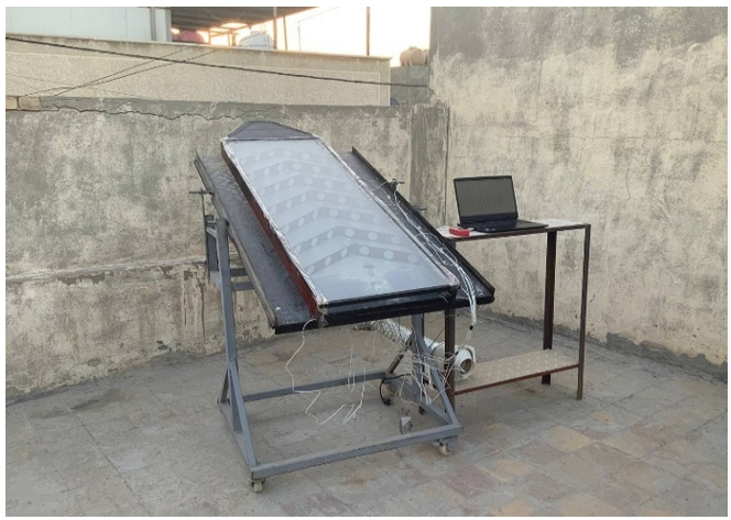
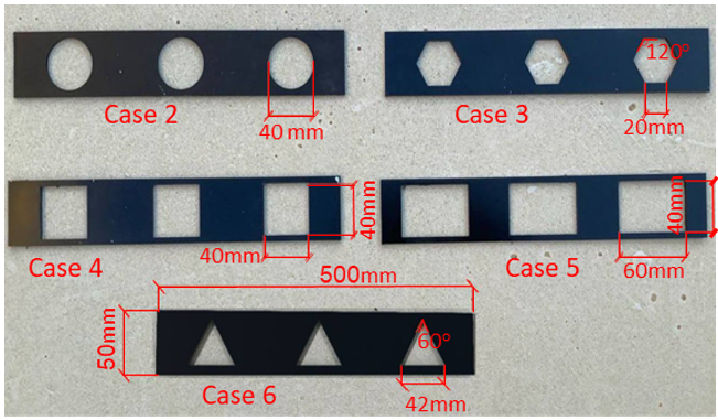
In this study, a SAH is utilized to convert solar energy into useful heat energy. The SAH is designed as perforated V-shaped barriers with different hole geometries, where it is tested experimentally [29]. Figure 1 shows the components of the SAH rig. Six scenarios are conducted experimentally in November in Baghdad. The average daily ambient air temperature during November was about 18 ℃, the average solar radiation for the same period was about 765 W/m2, and the average wind speed was about 1.2 m/s. The SAH consists of a rectangular duct that has dimensions of 1.5 m length, 0.5 m width, and 0.05 m height and is made from a wooden frame. The duct is covered topside by transparent glass. The absorbent plate is made of aluminum due to its high thermal convection coefficient of 871 J/Kg*K [30]. The dimensions of the absorber are 1.5 m, 0.5 m, and 0.003 m. It is coated with matte black paint, which is used to enhance heat absorption and improve heat transfer. The perforated barriers with various geometric designs are installed to investigate their effect on thermal and hydraulic performance. A blower is utilized to force air flow. The temperature is measured hourly by K-type thermocouples, which are fixed inside the duct and connected to an Arduino. The flow speed inside the duct is measured by an anemometer, while a digital manometer is employed to measure the pressure difference between the inlet and outlet of the duct. A solar meter is used to measure the value of solar radiation. The experiments are carried out, where six scenarios are considered to measure the improvement in the thermal performance of the SAH. These scenarios test the SAH with different geometries of perforated baffles inside the SAH duct, as shown in Figure 2, which shows the dimensions of each case. In this study, the SAH parameters are chosen depending on the previous studies [30-33]. The relative Roughness Pitch (p/e) is 3.5 and relative blockage height (e/H) is 1, the duct width to height ratio (W/H) is 10, and the angle of attack (α) is 60°. The scenarios of different barriers, which are shown in Figure 2, are:
•Scenario 1: without using SAH.
•Scenario 2: Used SAH 1 has a smooth absorbent plate as the reference case.
•Scenario 3: Used SAH 2 has V-dawn perforated baffles on an absorbent plate with circular holes.
•Scenario 4: Used SAH 3 has V-dawn perforated baffles on an absorbent plate with hexagonal holes.
•Scenario 5: Used SAH 4 has V-dawn perforated baffles on an absorbent plate with square holes.
•Scenario 6: Used SAH 5 has V-dawn perforated baffles on an absorbent plate with rectangular holes.
•Scenario 7: Used SAH 6 has V-dawn perforated baffles on an absorbent plate with triangular holes.
The heat transfer rate for SAH $H_{S A H}^t$ in (KW) can be expressed by [33-36]:
$H_{S A H}^t=m^{\circ} * C_p *\left(T_o-T_i\right)$ (1)
where, $m^{\circ}$ is mass flow rate in SAH duct in (Kg/s)$, Cp is Air specific heat in KJ/Kg*K and $T_o, T_i$ are average air outlet and inlet temperatures in $C^{\circ}$. In this study, the values of $H_{S A H}^t$ are measured experimentally and listed in Table 2.
Figure 1. Experimental test for solar air heaters (SAH)
Figure 2. Photo for cases barriers
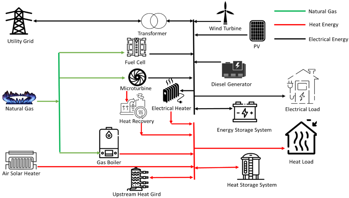
The structure of the proposed Smart MG based on CHP consists of MT, diesel generation DG, WT, photovoltaic panel PV, FC, and ESS, which is charged during off-peak time when the electrical price is lower and discharged to the system during peak hours. The CHP system also has an electrical heater EH, boiler heater, SAH, HSS to store heat, and HR to exploit heat from MT. In addition, the electrical power can be exchanged with the utility grid, and the heat system is connected with the district heating grid to share energy with the grid, to achieve the best performance operation. The proposed system is shown in Figure 3. The system modeling in this study was based on the literature.
Figure 3. Schematic diagram of combined heat and power microgrid (CHP-MG) and energy flow
3.1 Microturbines model
In this study, the mt is driven by natural gas to generate electricity. The mathematical relationship between electricity power generation and natural gas consumption in MT can be modeled by the linear equation [27, 37, 38]:
$C_{M T}^t=\frac{P_{M T}^t}{L C V * \eta_{M T}} * \lambda_g$ (2)
where, $C_{M T}$ the cost of fuel consumption by used MT in (\$), $L C V$ is the low heating value of natural gas $\left(\mathrm{kWh} / \mathrm{m}^3\right), \lambda_g$ is the price of natural gas $\left(\$ / \mathrm{m}^3\right), P_{M T}^t$ the output electrical power from MT at each time in kWh , and $\eta_{M T}$ it is efficiency of MT can be calculated by used [27]:
$\begin{aligned} \eta_{M T}= & 0.0753\left(\frac{P_{M T}^t}{65}\right)^3-0.3095\left(\frac{P_{M T}^t}{65}\right)^2 +0.1074\left(\frac{P_{M T}^t}{65}\right)+0.1068\end{aligned}$ (3)
The start-up cost $S U C_{M T}$ and shut-down cost $S D C_{M T}$ in $(\$)$ can be determined by:
$S U C_{M T}{ }^t=\mathrm{Sc}_{M T}\left(U_{M T}^t-U_{M T}^t * U_{M T}^{t-1}\right)$ (4)
$S D C_{M T}{ }^t=\mathrm{Sd}_{M T}\left(U_{M T}^{t-1}-U_{M T}^t * U_{M T}^{t-1}\right)$ (5)
The maintenance cost of MT $C_{\text {om.MT}}$ based on the maintenance cost rate coefficient $K_{\text {om.MT}}$ in ($/kWh) is calculated as in [37].
$C_{o m . M T}^t=P_{M T}^t * K_{o m . M T}$ (6)
3.2 Heat recovery model
The heat from the MT can be recovered using HR, where this heat can be expressed by the following equation $H_{M T}^t$ in (kW) by [39]:
$H_{M T}^t=\frac{P_{M T}^t\left(1-\eta_{M T}-\eta_l\right) \eta_{H R}}{\eta_{M T}}$ (7)
where, $\eta_l$ is the heat loss factor, $\eta_{H R}$ is the efficiency of HR.
3.3 Fuel cell model
The proton membrane FC is used to convert chemical energy stored in the gas into electrical energy. The $C_{F C}$ is the cost of fuel consumption by the used FC in (\$), $P_{F C}^t$ the output electrical power from FC at each time in (kWh), and $\eta_{F C}$ it is the efficiency of FC; the fuel consumption can be modeled by the linear equation [27, 37]:
$C_{F C}{ }^t=\frac{P_{F C}^t}{L C V * \eta_{F C}} * \lambda_g$ (8)
The start-up cost $S U C_{F C}$ and shut-down cost $S D C_{F C}$ in (\$) can be calculated by [35,38].
$S U C_{F C}{ }^t=\mathrm{Sc}_{F C}\left(U_{F C}^t-U_{F C}^t * U_{F C}^{t-1}\right)$ (9)
$S D C_{F C}{ }^t=\mathrm{Sd}_{F C}\left(U_{F C}^{t-1}-U_{F C}^t * U_{F C}^{t-1}\right)$ (10)
The maintenance cost of MT $C_{\text {om.FC}}$ based on the maintenance cost rate coefficient $K_{\text {OM.FC}}$ in ($/kWh) is calculated by the following equation [36]:
$C_{o m . F C}^t=P_{F C}^t * K_{o m . F C}$ (11)
3.4 Diesel generator model
The DG is an internal combustion engine which is driven by diesel fuel. The $C_{\mathrm{DG}}$ the cost of fuel consumption by the used DG in (\$), $P_{\mathrm{DG}}^t$ the output electrical power from FC at each time in (kWh), and $\eta_{\mathrm{DG}}$ it is the efficiency of DG; the fuel consumption can be modeled by the linear equation [37-41]:
$C_{\mathrm{DG}}{ }^t=a P_{\mathrm{DG}}^t{ }^2+b P_{\mathrm{DG}}^t+c$ (12)
where, a,b,c are cost coefficients of DG in ($/kW2h), (\$/kWh), (\$/h), respectively. The start-up cost $S U C_{D G}$ and shut-down $\operatorname{cost} S D C_{D G}$ in $(\$)$ can be determined by [36-40].
$S U C_{D G}{ }^t=\mathrm{Sc}_{D G}\left(U_{D G}^t-U_{D G}^t * U_{D G}^{t-1}\right)$ (13)
$S D U_{D G}^t=\operatorname{Sd}_{D G}\left(U_{D G}^{t-1}-U_{D G}^t * U_{D G}^{t-1}\right)$ (14)
The maintenance cost of DG $C_{\text {om.FC}}$ based on the maintenance cost rate coefficient $K_{o m . D G}$ in ($/kWh) [41].
$C_{o m . D G}^t=P_{D G}^t * K_{o m . D G}$ (15)
3.5 Wind turbine model
The power produced from the WT $P_{W T}^t$ in (kW) depends on the wind speed, and it can be calculated from the following equation [15, 16]:
$P_{W T}^t=\left\{\begin{array}{cc}0, & 0 \leq v_t<v_{\text {in}} \text { ot }>v_{\text {out}} \\ \frac{P_{W T}^R}{v_R^3-v_{\text {in}}^3} v_t^3-\frac{v_{\text {in}}^3}{v_R^3-v_{\text {in}}^3} P_{W T}^R & v_{\text {in}} \leq v_t \leq v_R \\ P_{W T}^R & v_R<v_t \leq v_{\text {out}}\end{array}\right.$ (16)
where, $P_{W T}^R$ is the rated output power from WT in (kW), $v_t$ is the wind speed in $(\mathrm{m} / \mathrm{s}), v_R$ is the rated wind speed of the WT, and $v_{\text {in}}, v_{\text {out}}$ are cut in wind speed and cut out wind speed, respectively.
3.6 Photovoltaic panel model
The PV is utilized to take advantage of solar energy by converting solar radiation into electric power $P_{P V}^t$ in (kW), it depends on solar radiation $I$ in $\mathrm{kW} / \mathrm{m}^2$. The total electrical power produced from PV $P_{P V}^t$ can be expressed by [15-17, 42]:
$P_{P V}^t=I^t *$ Area $P V * \eta_{P V} *$ number of $P V$ (17)
3.7 Solar air heater model
The SAH converts solar energy into useful heat energy. The heat transfer rate for SAH $H_{S A H}^t$ in (kW) can be expressed as Eq. (1).
3.8 Electrical heater model
The EH provides heat to supply heat load demand by converting electrical power to heat energy, where the output heat energy can be expressed $H_{E H}^t$ in (kW) by the following equation [35-37]:
$H_{E H}^t=P_{E H}^t * \eta_{E H}$ (18)
where, $P_{E H}^t$ is the electrical power consumed to produce heat by EH, and $\eta_{E H}$ is the efficiency of EH, and the maintenance cost of $\mathrm{EH} C_{\text {om.EK}}$ based on the maintenance cost rate coefficient $K_{o m . E H}$ in ($/kWh) [36-38].
$C_{o m . E H}^t=H_{E H}^t * K_{o m . E H}$ (19)
3.9 Gas boiler model
The GB generates heat by consuming natural gas. The cost of natural gas consumption in the GB to produce heat $C_{M T}$ in ($) can be determined by the following formula [26].
$C_{G B}{ }^t=\frac{H_{G B}^t}{L C V * \eta_{G B}} * p_g$ (20)
The maintenance cost of MT $C_{\text {om.MT}}$ based on the maintenance cost rate coefficient $K_{o m . M T}$ in ($/kWh) [36].
$C_{o m . G B}^t=H_{G B}^t * K_{o m . G B}$ (21)
3.10 Energy storage system model
ESS or Battery storage is used to store electrical power at times when energy is abundant, available, or cheap and store it for later use when energy is not available. It is useful in shifting energy from peak production times to peak consumption demand times, which increases the reliability and stability of the grid. The state of charge for the battery $S O C_b^t$ in (kWh) can be expressed by [11, 26, 27]:
$S O C_b^t=S O C_b^{t-1}-\frac{P_{b . d i s}^t}{\eta_{b . d i s}}+P_{b . c h}^t \eta_{b . c h}$ (22)
where, $P_{\text {b.ch}}^t, P_{\text {b.dis}}^t$ are the charging and discharging power of the battery in kWh , and $\eta_{c h}, \eta_{d i s}$ are the charging and discharging battery efficiency. The exchanged ESS power in kWh can be expressed by [35]:
$P_b^t=P_{b . d i s}^t-P_{b . c h}^t$ (23)
The $P_b^t$ it (+) at the discharge state where the ESS is purchasing to microgird, and (-) at the charging state where the battery consumes power. The cost of ESS during battery operation $C_b^t$ in \$ depends on the battery charge discharge prince $\lambda_b$ in (\$/kWh) is [38]:
$C_b^t=P_b^t * \lambda_b$ (24)
3.11 Heat storage system model
HSS, or a heat storage tank, stores heat. There are many ways to store heat, including the use of PCM [43, 44]. HSS is used to store heat power at times when it is available and store it for later use when the heat source is not available. It is useful in shifting energy from peak production times to peak consumption demand times, which increases the reliability of the grid. The state of charge for the battery $S O C_h^t$ in (kWh) can be expressed by [19, 25-39]:
$S O C_{h s}^t=S O C_{h s}^{t-1}-\frac{H_{h s . d i s}^t}{\eta_{h s . d i s}}+H_{h s . c h}^t \eta_{h s . c h}$ (25)
where, $H_{\text {hs.ch}}^t, H_{\text {hs.dis}}^t$ are the charging and discharging power HSS in kWh , and $\eta_{\text {hs.ch}}, \eta_{\text {hs.dis}}$ are the charging and discharging HSS efficiency. The exchanged HSS power in (kWh) can be expressed by [36]:
$H_{h s}^t=H_{h s . d i s}^t-H_{h s . c h}^t$ (26)
The $H_{h s}^t$ it (+) at the discharge state where the HSS purchasing to MG, and (-) at the charging state where HSS consumes power. The cost of HSS in the operation of the battery $C_{h s}^t$ in (\$) depends on the HSS charge discharge prince $\lambda_{h s}$ in (\$/kWh) is [37-39]:
3.12 Interacting power with the utility grid model
The proposed CHP system can exchange power with the utility grid to increase the reliability and stability of the grid as it shares energy with the grid according to the demand. It exports power when there is a surplus in electrical power production due to the availability of RE sources and imports power when electrical prices are low, and it is economical to import from the grid instead of operating production units or when there is a deficit in meeting demand [43]. The trading power $P_{U G}^t$ in (kWh) with the utility grid can be expressed by [37]:
$P_{U G}^t=P_{\text {import}}^t-P_{\text {export}}^t$ (28)
where, $P_{\text {import}}^t$ is import electrical power from grid in $(\mathrm{kWh})$, and $P_{\text {export}}^t$ is export electrical power to grid in $(\mathrm{kWh})$, the $P_{U G}^t$ t (+) at import purchasing state, and (-) at export selling. The power trading cost $C_{\text {e.UG}}^t$ in (\$) depends on the electrical prince $\lambda_{\text {elect} .}^t$ in ($/kWh) is:
$C_{\text {e.UG}}^t=P_{U G}^t * \lambda_{\text {elect}}^t$. (29)
The constraint capacity of the interacting power it can be expressed by [11, 36]:
$P_{\text {import}}^{m i n} U_{\text {e.import}}^t \leq P_{\text {import}}^t \leq P_{\text {import}}^{m a s} U_{\text {e.import}}^t$ (30)
$P_{\text {export}}^{\min} U_{\text {e.export}}^t \leq P_{\text {export}}^t \leq P_{\text {export}}^{\text {mas}} U_{\text {e.export}}^t$ (31)
$U_{\text {e.import}}^t+U_{\text {e.export}}^t \leq 1$ (32)
where, $P_{\text {import}}^{\min}, P_{\text {import}}^{\text {mas}}$ limit power can be imported and $U_{\text {e.import}}^t$ electrical import on/ off state. And where $P_{\text {export}}^{\text {min}}, P_{\text {export}}^{\text {mas}}$ limit power can be exported and $U_{\text {e.export}}^t$ electrical export on/ off state.
3.13 Exchanging heat power with the upstream grid model
The CHP system can trade heat energy with the upstream gird or to increase the reliability gird as it shares heat energy with the gird according to the demand response, exports heat power when there is a surplus in heat power and import heat when heat prices are low and it is economical to import from the gird instead of operating production units or when there is a deficit in meeting demand [43]. The trading power $H_{U G}^t$ in (kWh) with the utility grid can be expressed by [36, 37]:
$H_{U G}^t=H_{\text {import}}^t-H_{\text {export}}^t$ (33)
where, $H_{\text{import}}^t$ is import heat power from the grid in (kWh) and $H_{\text {export}}^t$ is the heat electrical power to grid in (kWh), the $H_{U G}^t$ t (+) at import purchasing state, and (–) at export selling. The power heat trading cost $C_{\text{h,UG}}^t$ in (\$) depends on the electrical prince $\lambda_{\text{heat}}^t$ in (\$/kWh) is [37]:
$C_{\text {h.UG}}^t=H_{U G}^t * \lambda_{\text {heat}}^t$. (34)
3.14 Emission cost model
GHG emissions such as CO2, SO2, NOx, and PM are emitted during the energy production process. It is important to reduce these emissions to the minimum possible level. Therefore, the emitted gases are considered as a cost in the cost objective function according to the monetary concept. The total emission cost $C_{E m i .}^t$ in ($) can be expressed by:
$C_{E m i .}^t=\sum_1^i \sum_1^j P_i^t C_j E_{i, j}$ (35)
where, $P_i^t(\mathrm{kWh})$ in is the generated power from DG, MT, and FC. The Cj in (\$/kg) is the expense of the emission price of $j^{\text {th}}$ GHG. The $E_{i, j}$ in (kg/kWh) is the amount of emissions $j^{\text {th}}$ GHGs from $i^{\text {th}}$ generators [25].
In this study, the multi objective optimization problem [44] is converted to a single objective that can be solved in one step by converting the emission of GHGs into a monetary concept. This function includes all the aforementioned costs as in the following equation.
$\begin{aligned} C F=\min & \sum_{t=1}^{24}\left[C_{M T}^t+C_{o m . M T}^t+S U C_{M T}{ }^t+S D C_{M T}{ }^t\right. \\ +C_{F C}{ }^t & +S U C_{F C}{ }^t+S D C_{F C}{ }^t+C_{o m . F C}^t+C_{\mathrm{DG}}{ }^t \\ +S U C_{D G}{ }^t & +S D U_{D G}^t+C_{o m . D G}^t+C_{G B}{ }^t+C_{o m . G B}^t+C_b^t \\ & \left.+C_{h s}^t+C_{e . U G}^t+C_{h . U G}^t+C_{E m i .}^t\right]\end{aligned}$ (36)
The objective function is subject to the constraints that limit the operation of the energy resources. These constraints should be met at each time interval. These constraints are as follows:
5.1 Microturbines constraints
The capacity constraint of the MT can be expressed as follows [35-39]:
$P_{M T}^{\min } U_{M T}^t \leq P_{M T}^t \leq P_{M T}^{\max } U_{M T}^t$ (37)
where, $P_{M T}^{\text {min}}, P_{M T}^{\text {max}}$ is the minimum and maximum power that can be produced by MT in (kW), and the $U_{M T}$ on/off state of MT, and the ramp rate constraint for MT at each time interval should be the ramp-up limit $U R_{M T}$ and ramp-down limit $D R_{M T}$ in (kW) [12, 37 ].
$P_{M T}^t-P_{M T}^{t-1} \leq U R_{M T}$ (38)
$P_{M T}^{t-1}-P_{M T}^t \leq D R_{M T}$ (39)
5.2 Fuel cell constraints
The capacity constraint of the FC can be expressed as follows:
$P_{F C}^{\min } U_{F C}^t \leq P_{F C}^t \leq P_{F C}^{\max } U_{F C}^t$ (40)
where, $P_{F C}^{\text {min}}, P_{F C}^{\text {max}}$ is the minimum and maximum power that can be produced by FC in (kW), and the $U_{F C}$ on/off state of FC, and the ramp rate constraint for FC at each time interval should be the ramp-up limit $U R_{F C}$ and ramp-down limit $D R_{F C}$ in (kW) [13].
$P_{F C}^t-P_{F C}^{t-1} \leq U R_{F C}$ (41)
$P_{F C}^{t-1}-P_{F C}^t \leq D R_{F C}$ (42)
5.3 Diesel generator constraints
The capacity constraint of DE can be determined using the following equation:
$P_{D G}^{\min } U_{D G}^t \leq P_{b . c h}^t \leq P_{D G}^{\max } U_{D G}^t$ (43)
where, $P_{D G}^{\text {min}}, P_{D G}^{\text {max}}$ is the minimum and maximum power that can be produced by DG in (kW), and the $U_{D G}$ on/off state of DG, and the ramp rate constraint for FC at each time interval should be the ramp-up limit $U R_{D G}$ and ramp-down limit $D R_{D G}$ in (kW) [42, 45].
$P_{D G}^t-P_{D G}^{t-1} \leq U R_{D G}$ (44)
$P_{D G}^{t-1}-P_{D G}^t \leq D R_{D G}$ (45)
5.4 Electrical heater constraints
The constraint of the capacity of the EH can be determined using the following formula:
$H_{E H}^{\min} U_{E H}^t \leq H_{E H}^t \leq H_{E H}^{\max} U_{E H}^t$ (46)
where, $H_{E H}^{\text {min}}, H_{E H}^{\text {max}}$ is the minimum and maximum power that can be produced by EH in (kW), and the $U_{E H}$ on/off state of EH [38].
5.5 Gas boiler constraints
The constraint of the GB can be expressed by:
$H_{G B}^{\min} U_{G B}^t \leq H_{G B}^t \leq H_{G B}^{\max} U_{G B}^t$ (47)
where, $H_{G B}^{\text {min}}, H_{G B}^{\text {max}}$ is the minimum and maximum power that can be produced by FC in (kW), and the $U_{G B}$ on/off state of GB [35-38].
5.6 Energy storage system constraints
The constraint of the operation of the battery can be expressed as follows:
$P_b^{\min} \leq P_b^t \leq P_b^{\max}$ (48)
$P_{b . c h}^{\min } U_{b . c h}^t \leq P_{b . c h}^t \leq P_{b . c h}^{\max } U_{b . c h}^t$ (49)
$P_{\text {b.dis}}^{\min} U_{\text {b.ch}}^t \leq P_{\text {b.dis}}^t \leq P_{\text {b.dis}}^{\max} U_{\text {b.dis}}^t$ (50)
$U_{b . d i s}^t+U_{b . c h}^t \leq 1$ (51)
where, the $P_{b . c h}^{\min}, P_{b . d i s}^{\min}$ are the minimum limit charge and discharge power battery in (kW), and $P_b^{\text {max}}, P_b^{\text {min}}$ are limits of battery capacity, and $P_{\text {b.ch}}^{\text {max}}, P_{\text {b.dis }}^{\text {max}}$ are the maximum limit charge and discharge power battery in (kW), and where $U_{\text {b.ch}}^t$, $U_{\text {b.dis}}^t$ are on/ off state of charge and discharge [38-40].
5.7 Heat storage system constraints
The constraint of the operation of the heat storage can be determined using the expression below:
$H_{h s}^{\min} \leq H_{h s}^t \leq H_{h s}^{\max}$ (52)
$H_{h s . c h}^{\min} U_{h s . c h}^t \leq H_{h s . c h}^t \leq H_{h s . c h}^{\max} U_{h s . c h}^t$ (53)
$H_{h s . d i s}^{\min} U_{h s . c h}^t \leq H_{h s . d i s}^t \leq H_{h s . d i s}^{\max} U_{h s . d i s}^t$ (54)
$U_{h s . d i s}^t+U_{h s . c h}^t \leq 1$ (55)
where, the $H_{\text {hs.ch }}^{\min}, H_{\text {hs.dis }}^{\min}$ are the minimum limit charge and discharge power battery in (kW), and $H_{h s}^{\text {max}}, H_{h s}^{\text {min}}$ are the limits of HSS capacity, and $H_{\text {hs.ch}}^{m a x}, H_{\text {hs.dis}}^{m a x}$ are the maximum limit charge and discharge power of HSS in (kW), and where $U_{\text {hs.ch}}^t, U_{\text {hs.dis}}^t$ are on/ off state of charge and discharge [36-38].
5.8 Heat power with the upstream grid constraints
The constraint capacity of the interacting heat power can be expressed as follows:
$H_{\text {import}}^{\text {min}} U_{\text {h.import}}^t \leq H_{\text {import}}^t \leq H_{\text {import}}^{\text {mas}} U_{\text {h.import}}^t$ (56)
$H_{\text {export}}^{\min} U_{\text {h.export}}^t \leq H_{\text {export}}^t \leq H_{\text {export}}^{\operatorname{mas}} U_{\text {h.export}}^t$ (57)
$U_{\text {h.import}}^t+U_{\text {h.export}}^t \leq 1$ (58)
where, $H_{\text {import}}^{\min}, H_{\text {import}}^{\operatorname{mas}}$ limit power can be imported and $U_{\text {e.import}}^t$ heat import on/ off state. And where $H_{\text {export}}^{\text {min}}$, $H_{\text {export}}^{\text {mas}}$ limit power can be exported and $U_{\text {h.export}}^t$ heat export on/off state [35-37].
5.9 Power balance constraint model
In order to ensure the production of electrical and heat energies that covers the required electrical and heat demand loads for each period, this constraint should be considered:
$\begin{gathered}P_{M T}^t+P_{F C}^t+P_{D G}^t+P_{P V}^t+P_{W T}^t+P_{\text {b.dis}}^t+P_{\text {import}}^t =P_{\text {export}}^t+P_{\text {b.ch}}^t+P_{E H}^t+L_{\text {elctr}}^t .\end{gathered}$ (59)
where, $L_{\text {elctr} .}^t$ it is the electrical power demand load in (kWh).
$\begin{gathered}H_{M T}^t+H_{G B}^t+P_{\text {SAH}}^t+H_{E H}^t+H_{\text {b.dis}}^t+H_{\text {import}}^t =H_{\text {export}}^t+H_{\text {b.ch}}^t+L_{\text {heat.}}^t\end{gathered}$ (60)
where, $L_{\text {heat.}}^t$ it is heating power demand load in (kWh).
The proposed system under study, which is shown in Figure 3 consisting of electrical loads and thermal loads and contains FC, MT, and DG to cover electrical loads, and GB, EH, and HR systems from MT to cover thermal loads. Table 1 list the hourly values of the loads, price, RE generation, and heat from the SAH. It is considered that 100 SAH are exist. Seven scenarios are tested, where scenario 1 is without SAH, and scenarios 2–7 use SAH in various SAH types. The heat energy output from the SAHs is shown in Table 2. Thermal and electrical storage system characteristics are listed in Table 3, while the emission cost parameters are in Table 4. The technical parameters of conventional energy sources are as in Table 5. The minimum and maximum of exchanging electric and heat energies are 10 and 200 kWh, respectively. The efficiencies of electric and HSSs are considered 90%. While the minimum and maximum charging and discharging power are 90 kWh. The minimum and maximum state of charge for electric and HSSs are 90 and 300 kWh, respectively. The natural gas cost prince $\lambda_g$ was 0.3 $/m3, have LCV was 9.78 kWh/m3. This grid has 100 PVs, have efficiency $\eta_{P V}$ 24%; PV area for each PV was 2.374 m2. HR system efficiency $\eta_{H R}$ was 75%, heat loss factor was $\eta_l$ 20%.
Table 1. Hourly loads, prices, and renewable generation
|
Time (h) |
$L_{\text {elctr.}}^t$ (kWh) |
$L_{\text {heat.}}^t$ (kWh) |
$\lambda_{\text {elect.}}^t$ ($/kWh) |
$\lambda_{\text {heat.}}^t$ ($/kWh) |
$P_{W T}^t$ (kW) |
$I^t$ kW/m2 |
|
t1 |
192 |
466.88 |
0.01 |
0.162 |
55 |
0 |
|
t2 |
177.6 |
481.82 |
0.018 |
0.1332 |
61 |
0 |
|
t3 |
132 |
489.29 |
0.02 |
0.1368 |
65 |
0 |
|
t4 |
122.4 |
481.82 |
0.018 |
0.1476 |
58 |
0 |
|
t5 |
117.6 |
489.29 |
0.025 |
0.1008 |
58 |
0 |
|
t6 |
110.4 |
451.94 |
0.045 |
0.054 |
24 |
0.100 |
|
t7 |
162 |
443.22 |
0.1 |
0.0432 |
40 |
0.200 |
|
t8 |
213.6 |
428.28 |
0.28 |
0.0972 |
34 |
0.600 |
|
t9 |
258 |
382.22 |
0.45 |
0.1152 |
40 |
0.655 |
|
t10 |
220.8 |
343.62 |
0.519 |
0.144 |
46 |
0.810 |
|
t11 |
295.2 |
336.15 |
0.4 |
0.1116 |
30 |
0.890 |
|
t12 |
368.4 |
290.09 |
0.25 |
0.09 |
31 |
0.950 |
|
t13 |
442.8 |
252.74 |
0.48 |
0.054 |
25 |
0.900 |
|
t14 |
421.2 |
217.88 |
0.3 |
0.054 |
25 |
0.780 |
|
t15 |
406.8 |
244.02 |
0.25 |
0.0792 |
36 |
0.630 |
|
t16 |
368.4 |
282.662 |
0.1 |
0.126 |
30 |
0.480 |
|
t17 |
327.6 |
367.28 |
0.035 |
0.1476 |
46 |
0.020 |
|
t18 |
339.6 |
428.28 |
0.045 |
0.1152 |
36 |
0 |
|
t19 |
361.2 |
520.41 |
0.08 |
0.1008 |
52 |
0 |
|
t20 |
420 |
573.95 |
0.12 |
0.0972 |
46 |
0 |
|
t21 |
405.6 |
559.01 |
0.025 |
0.1584 |
52 |
0 |
|
t22 |
421.2 |
555.27 |
0.015 |
0.1476 |
46 |
0 |
|
t23 |
375.6 |
539.09 |
0.012 |
0.108 |
46 |
0 |
|
t24 |
370.8 |
520.41 |
0.01 |
0.288 |
52 |
0 |
Table 2. Output heat power from solar air heater (SAH) cases in KW
|
SAH 1 |
SAH 2 |
SAH 3 |
SAH 4 |
SAH 5 |
SAH 6 |
|
|
t1 |
0 |
0 |
0 |
0 |
0 |
0 |
|
t2 |
0 |
0 |
0 |
0 |
0 |
0 |
|
t3 |
0 |
0 |
0 |
0 |
0 |
0 |
|
t4 |
0 |
0 |
0 |
0 |
0 |
0 |
|
t5 |
0 |
0 |
0 |
0 |
0 |
0 |
|
t6 |
0.08 |
0.1 |
0.1 |
0.1 |
0.1 |
0.1 |
|
t7 |
0.1 |
0.13 |
0.27 |
0.29 |
0.173 |
0.3 |
|
t8 |
0.12 |
0.3 |
0.3 |
0.42 |
0.25 |
0.38 |
|
t9 |
0.13 |
0.44 |
0.4 |
0.49 |
0.47 |
0.48 |
|
t10 |
0.17 |
0.47 |
0.65 |
0.53 |
0.51 |
0.64 |
|
t11 |
0.27 |
0.58 |
0.67 |
0.6 |
0.59 |
0.65 |
|
t12 |
0.35 |
0.59 |
0.68 |
0.61 |
0.604 |
0.651 |
|
t13 |
0.34 |
0.6 |
0.66 |
0.6 |
0.58 |
0.647 |
|
t14 |
0.34 |
0.58 |
0.65 |
0.59 |
0.57 |
0.62 |
|
t15 |
0.32 |
0.5 |
0.62 |
0.56 |
0.54 |
0.58 |
|
t16 |
0.17 |
0.43 |
0.6 |
0.5 |
0.43 |
0.54 |
|
t17 |
0.1 |
0.15 |
0.5 |
0.45 |
0.23 |
0.52 |
|
t18 |
0.07 |
0.01 |
0.25 |
0.2 |
0.1 |
0.1 |
|
t19 |
0 |
0 |
0.1 |
0.1 |
0.08 |
0 |
|
t20 |
0 |
0 |
0 |
0 |
0 |
0 |
|
t21 |
0 |
0 |
0 |
0 |
0 |
0 |
|
t22 |
0 |
0 |
0 |
0 |
0 |
0 |
|
t23 |
0 |
0 |
0 |
0 |
0 |
0 |
|
t24 |
0 |
0 |
0 |
0 |
0 |
0 |
Table 3. Energy and heat storage system (HSS) parameters
|
Type |
$P_{c h}^{\max}$ (kW) |
$P_{c h}^{\text {min}}$ (kW) |
$P_{\text {dis }}^{\max}$ (kW) |
$P_{\text {dis }}^{\min}$ (kW) |
$P^{\text {max}}$ (kW) |
$P^{\text {min}}$ (kW) |
$\eta_{c h}$ |
$\boldsymbol{\eta}_{\text {dis}}$ |
$\lambda$ ($/kWh) |
|
ESS |
90 |
5 |
90 |
5 |
300 |
90 |
0.9 |
0.9 |
0.06 |
|
HSS |
90 |
5 |
90 |
5 |
300 |
90 |
0.9 |
0.9 |
0.0031 |
Table 4. Emission parameters
|
Source |
$E_{\text {CO2}}$ (kg/kWh) |
$E_{\text {NOx}}$ (kg/kWh) |
$E_{\text {SO2}}$ (kg/kWh) |
$E_{P M}$ (kg/kWh) |
|
DG |
0.848 |
0.0013 |
0.00125 |
0.00036 |
|
FC |
0.489 |
0.00001 |
0.000003 |
0.000001 |
|
MT |
0.725 |
0.0002 |
0.000004 |
0.000041 |
|
$C_j$ ($/kg) |
0.02 |
5 |
6 |
25 |
Table 5. Conventional power and heat energy sources work by fuel burn parameters
|
Elect. |
$P_i^{\min}$ kW |
$P_i^{\text {max}}$ kW |
$\eta_i$ |
$K_{\text {om} . i}$ $/kWh |
Sci ($) |
Sdi ($) |
$U R_i$ (kW) |
$D R_i$ (kW) |
a $/kW2h |
b $/kWh |
c ($/h) |
|
DG |
20 |
200 |
- |
0.01258 |
0.25 |
0.25 |
100 |
100 |
0.006 |
1 |
10 |
|
MT |
20 |
200 |
0.3 |
0.026 |
0.1 |
0.1 |
100 |
100 |
- |
- |
- |
|
FC |
10 |
40 |
0.6 |
0.026 |
0.2 |
0.1 |
20 |
20 |
- |
- |
- |
|
HEAT |
$H_i^{\text {min}}$ (kW) |
$H_i^{\max}$ (kW) |
$\eta_i$ |
$K_{\text {om.i }}$ $/kWh |
Sci ($) |
Sdi($) |
$U R_i$ (kW) |
$D R_i$ (kW) |
a ($/kW2h) |
b ($/kWh) |
c ($/h) |
|
GB |
0 |
100 |
0.73 |
0.0027 |
- |
- |
- |
- |
- |
- |
- |
|
EH |
0 |
500 |
0.8 |
0.002 |
- |
- |
- |
- |
- |
- |
- |
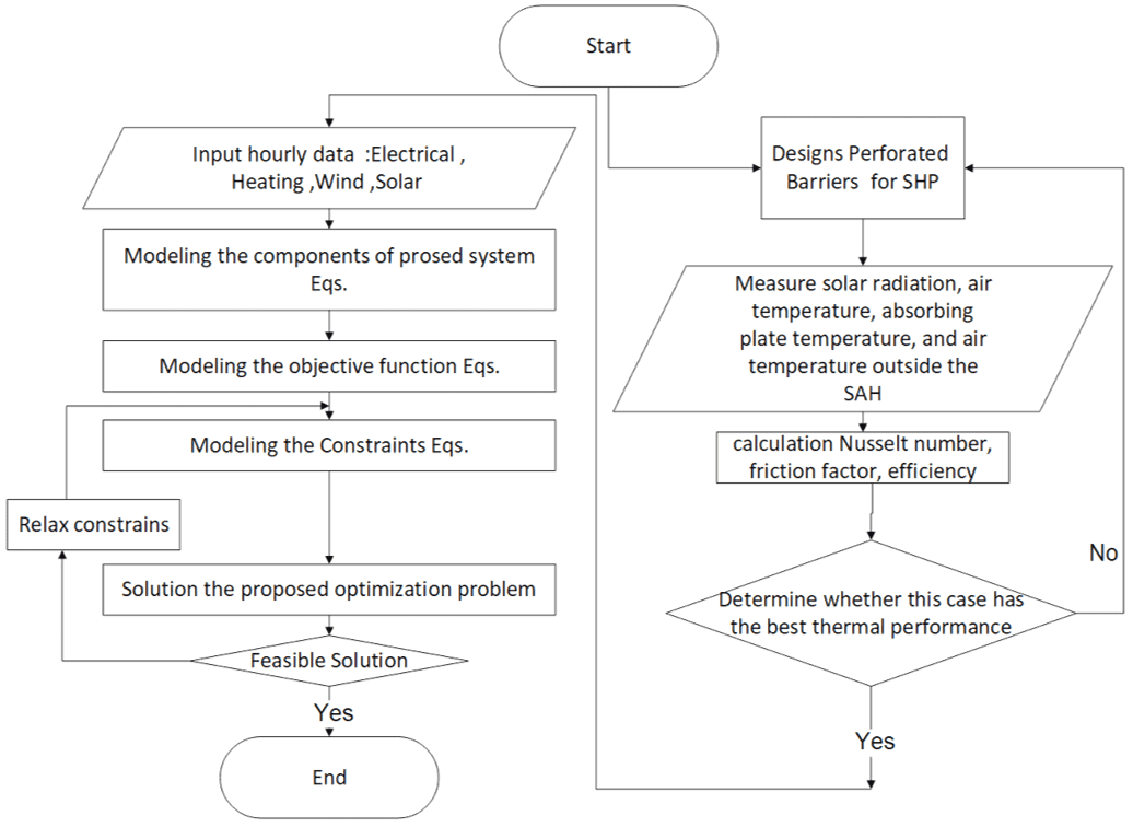
The formulation of the optimization problem is formulated as UCMOMINL, where the problem includes both continuous and integer variables. The emission level of the GHGs is converted to a monetary concept form and integrated with the objective function in one entire framework, and the problem is converted to a single function that can be solved directly in one step. General Algebraic Modelling System (GAMS) software is employed to formulate and model the proposed optimization problem. Gams is a highly mathematical modelling system for modelling and solving optimization problems. The MINLP solver with interfacing with Microsoft Excel is employed to solve the proposed optimization problem. The flowchart shown in Figure 4 shows the process that has been followed to formulate and solve the proposed approach.
Figure 4. Flowchart of the formulation of and solution to the proposed optimization problem
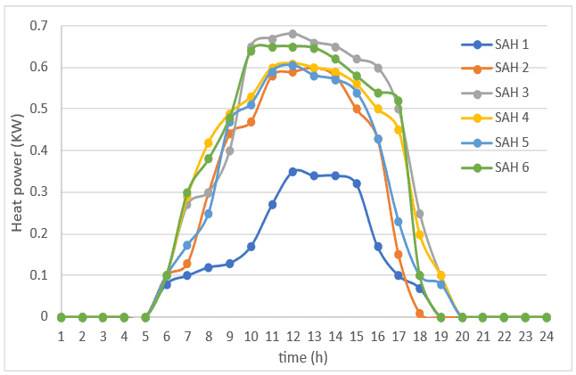
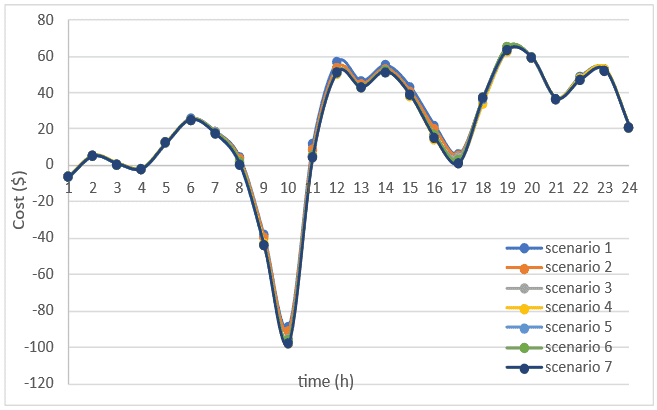
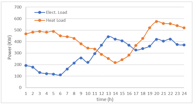
Seven scenarios of SAH improvement have been experimentally conducted. These scenarios were carried out during November in Baghdad. Six scenarios of SAH output heat energy are depicted in Figure 2, while scenario 1 is without SAH. The best scenario is scenario 4, where the total daily cost is 437.38\$, while it is 439.97\$ of scenario 7. The cost is 441.86\$ for scenario 5, and scenario 6 has a total cost 450.4\$. The total cost of scenario 3 is 454.54\$, while scenario 2 has a total cost 477.5\$. The worst scenario was scenario 1 have total cost 500.34\$. The use of SAH has reduced the operational cost, as it provides free heat in addition to increasing the diversity of sources, which enhances grid flexibility. Table 2 and Figure 5 show the hourly output heat energy of the SAH for the six scenarios, while Figure 6 depicts the hourly total cost of the six scenarios and Table 6 lists the hourly output energy of the seven scenarios. As the hourly electric and heat loads load in Figure 7. This is due to the distinctive designs of the perforated, it had the best thermal performance for the case SAH 3, which has hexagonal holes, which increased air turbulence and raised the Nusselt number value without increasing the Fracture Factor significantly, and produced the highest heat power; for this it was the scenario 4 was the best cost.
Figure 5. Output heat power by solar air heaters (SAH)
Figure 6. Hourly total cost for each scenario
Table 6. Hourly total cost for each scenario in ($)
|
Time (h) |
Scenario 1 |
Scenario 2 |
Scenario 3 |
Scenario 4 |
Scenario 5 |
Scenario 6 |
Scenario 7 |
|
t1 |
-6.02559 |
-6.02559 |
-6.02559 |
-6.02559 |
-6.02559 |
-6.02559 |
-6.02559 |
|
t2 |
5.371149 |
5.371149 |
5.371149 |
5.371149 |
5.371149 |
5.371149 |
5.371149 |
|
t3 |
1.022277 |
1.022277 |
1.022277 |
1.022277 |
1.022277 |
1.022277 |
1.022277 |
|
t4 |
-1.56317 |
-1.56317 |
-1.56317 |
-1.56317 |
-1.56317 |
-1.56317 |
-1.56317 |
|
t5 |
12.63233 |
12.63233 |
12.63233 |
12.63233 |
12.63233 |
12.63233 |
12.63233 |
|
t6 |
25.9891 |
25.5571 |
25.4491 |
25.4491 |
25.4491 |
25.4491 |
25.4491 |
|
t7 |
18.98779 |
18.54059 |
18.40643 |
17.78034 |
17.6909 |
18.21413 |
17.64618 |
|
t8 |
4.783566 |
3.617166 |
1.867566 |
1.867566 |
0.701166 |
2.353566 |
1.089966 |
|
t9 |
-38.0461 |
-39.5437 |
-43.1149 |
-42.6541 |
-43.6909 |
-43.4605 |
-43.5757 |
|
t10 |
-88.422 |
-90.87 |
-95.19 |
-97.782 |
-96.054 |
-95.766 |
-97.638 |
|
t11 |
11.9096 |
8.896402 |
5.436802 |
4.432402 |
5.213602 |
5.325202 |
4.655602 |
|
t12 |
56.98502 |
53.83502 |
51.67502 |
50.86502 |
51.49502 |
51.54902 |
51.12602 |
|
t13 |
46.54342 |
44.64005 |
43.23605 |
42.91205 |
43.23605 |
43.34405 |
42.98225 |
|
t14 |
55.19085 |
53.35485 |
52.05885 |
51.68085 |
52.00485 |
52.11285 |
51.84285 |
|
t15 |
43.38071 |
40.84631 |
39.42071 |
38.47031 |
38.94551 |
39.10391 |
38.78711 |
|
t16 |
22.27928 |
20.13728 |
16.86128 |
14.71928 |
15.97928 |
16.86128 |
15.47528 |
|
t17 |
6.315512 |
5.866372 |
5.128372 |
1.516891 |
1.532391 |
3.011212 |
1.510691 |
|
t18 |
37.35406 |
37.52128 |
37.23886 |
34.47406 |
36.58828 |
37.74028 |
37.74028 |
|
t19 |
65.47691 |
65.47691 |
65.47691 |
63.06104 |
63.7098 |
65.50171 |
63.82153 |
|
t20 |
59.25296 |
59.25296 |
59.25296 |
59.25296 |
59.25296 |
59.25296 |
59.25296 |
|
t21 |
36.97853 |
36.97853 |
36.97853 |
36.97853 |
36.97853 |
36.97853 |
36.97853 |
|
t22 |
49.40867 |
47.77629 |
48.38181 |
48.38181 |
47.42516 |
47.42516 |
47.42516 |
|
t23 |
53.17577 |
52.81415 |
53.17577 |
53.17577 |
52.60445 |
52.60445 |
52.60445 |
|
t24 |
21.36524 |
21.36524 |
21.36524 |
21.36524 |
21.36524 |
21.36524 |
21.36524 |
|
total |
500.345 |
477.499 |
454.542 |
437.384 |
441.864 |
450.403 |
439.976 |
Table 7. Hourly cost for scenarios 1 and 4 in ($)
|
Scenario 1 |
Scenario 4 |
|||||
|
Time (h) |
Electrical Cost |
Heat Cost |
Emission Cost |
Electrical Cost |
Heat Cost |
Emission Cost |
|
t1 |
20.187 |
-27.212 |
1 |
20.187 |
-27.212 |
1 |
|
t2 |
21.787 |
-17.416 |
1 |
21.787 |
-17.416 |
1 |
|
t3 |
22.187 |
-22.164 |
1 |
22.187 |
-22.164 |
1 |
|
t4 |
21.787 |
-24.350 |
1 |
21.787 |
-24.350 |
1 |
|
t5 |
23.187 |
-11.554 |
1 |
23.187 |
-11.554 |
1 |
|
t6 |
10.873 |
15.116 |
0 |
10.873 |
14.576 |
0 |
|
t7 |
5.347 |
12.641 |
1 |
5.347 |
11.433 |
1 |
|
t8 |
-8.297 |
12.081 |
1 |
-8.297 |
9.165 |
1 |
|
t9 |
-40.975 |
1.929 |
1 |
-40.975 |
-2.679 |
1 |
|
t10 |
-80.294 |
-9.128 |
1 |
-80.294 |
-18.488 |
1 |
|
t11 |
7.983 |
2.926 |
1 |
7.983 |
-4.551 |
1 |
|
t12 |
56.905 |
-0.920 |
1 |
56.905 |
-7.040 |
1 |
|
t13 |
41.117 |
4.426 |
1 |
41.117 |
0.795 |
1 |
|
t14 |
51.714 |
2.477 |
1 |
51.714 |
-1.033 |
1 |
|
t15 |
41.913 |
0.468 |
1 |
41.913 |
-4.443 |
1 |
|
t16 |
25.292 |
-4.013 |
1 |
25.292 |
-11.573 |
1 |
|
t17 |
25.187 |
-19.871 |
1 |
25.187 |
-24.670 |
1 |
|
t18 |
30.387 |
5.967 |
1 |
30.387 |
3.087 |
1 |
|
t19 |
39.587 |
24.890 |
1 |
37.259 |
24.802 |
1 |
|
t20 |
34.267 |
23.986 |
1 |
34.267 |
23.986 |
1 |
|
t21 |
23.187 |
12.792 |
1 |
23.187 |
12.792 |
1 |
|
t22 |
21.187 |
27.222 |
1 |
21.187 |
26.195 |
1 |
|
t23 |
25.987 |
26.189 |
1 |
25.987 |
26.189 |
1 |
|
t24 |
20.187 |
0.179 |
1 |
20.187 |
0.179 |
1 |
|
total |
440.685 |
36.66 |
23 |
438.357 |
-23.973 |
23 |
Figure 7. Hourly electric and heat loads
Figure 8. Optimal heat power schedule with heat load scenario 1
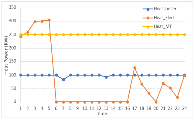
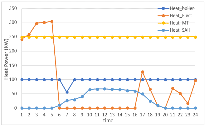
Comparing scenario 4, which is the best scenario, with scenario 1, which is the reference Scenario. It can be seen that the total cost reduces by 12.58% in the case of scenario 4. The optimal schedules of heat energy resources for both scenarios are close, with a slight difference at t19, where the EH output heat increases in scenario 1 to compensate for the heat loss, as shown in Figures 8 and 9. Besides, the presence of the SAH reduces the heat cost very significantly, and there is surplus heat that is exported to the grid. This achieves a profit from heat sales, which leads to a reduction in the total system cost by 62.96$ as shown in Tables 6 and 7.
Figure 9. Optimal heat power schedule with heat Load scenario 4
Figure 10. Optimal electrical power schedule of scenario 1
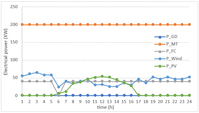
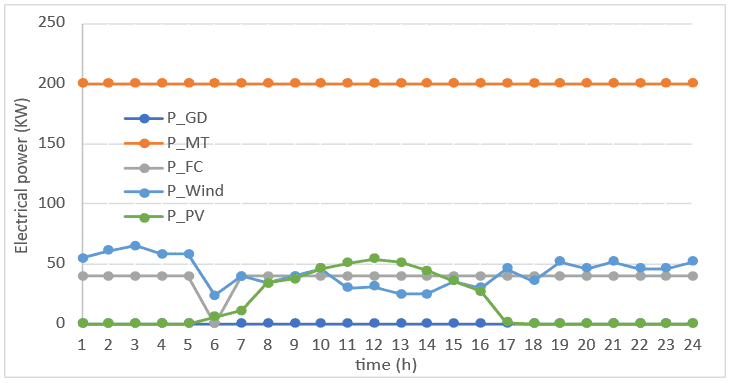
Figures 10 and 11 show the optimal production of electrical energy sources for scenarios 1 and 4. It can be seen that both schedules in both scenarios are close. DG is in the off state at all times due to its high operating cost, while the production of electrical energy from MT supplies the highest possible power due to its low cost and to supply heat to the heat grid in addition to supplying the electric load. The rest of the energy is supplied by the presence of renewable sources. In addition, it can be observed that the FC is turned off at t6 because the electric load has the lowest value at this hour and the price reaches a low value.
Figure 11. Optimal electrical power schedule of scenario 4
Figure 12. Optimal power schedule of energy storage system (ESS) scenario 1
Figure 13. Optimal power schedule of energy storage system (ESS) scenario 4
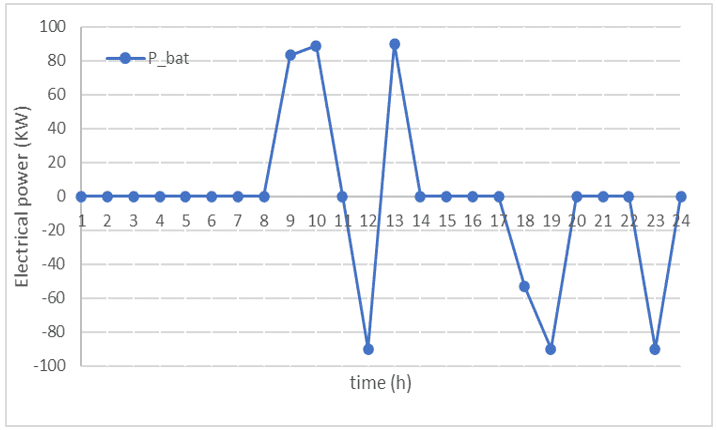
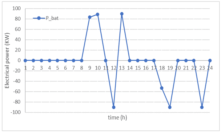
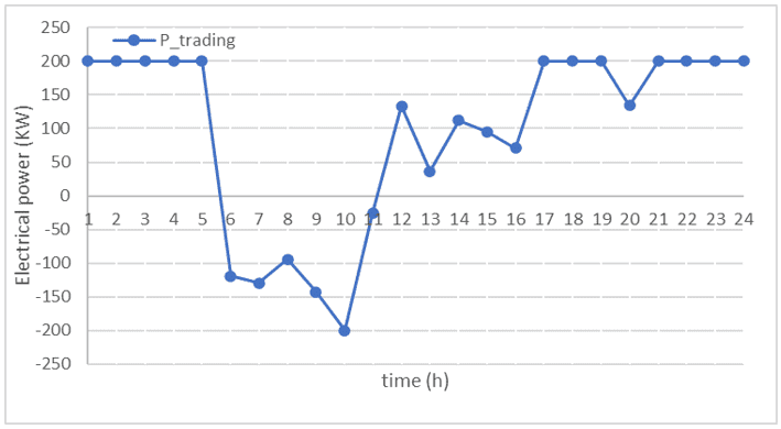
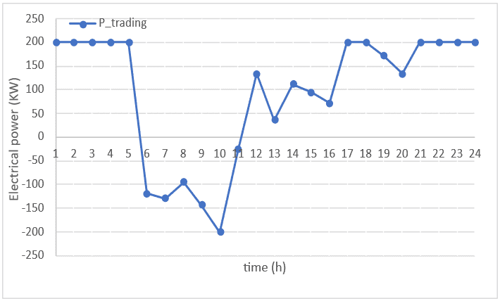
The battery is discharged during t8, t9, and t13 to contribute to supplying the loads and to sell power to the grid because the electrical price has high values at these hours. The battery is charged at t12 because the renewable energies have the highest generation at this hour, where the battery stores this energy and discharges it during high demand. The battery is also charged at t17 and t23 to its maximum state of charge because the price has low values and meets the constraints to fully charge the battery at the end of the scheduling day, as shown in Figures 12 and 13. During the day, electrical energy is imported and exported from the network, relying on the price difference to achieve maximum profit, as in Figures 14 and 15. In both scenarios, the amount of exchange is close, with slight differences as a result of the addition of SAH, which reduces the operation of the electric heater.
Figure 14. Optimal exchange power with the utility grid scenario 1
Figure 15. Optimal exchange power with the utility grid scenario 4
Figure 16. Heat power exchange with grid scenario 1
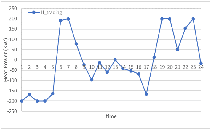
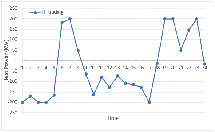
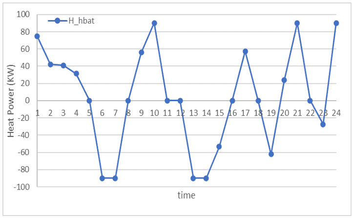
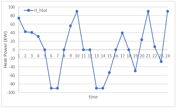
Similarly for the heat grid, the optimal schedule of heat energy sources is shown in Figures 8 and 9. The load is covered by recovering the waste heat from the MT, while the remaining load is covered by the GB, and during peak heat demand times during the period t1–t6, t16–t24, the EH will work to cover the remaining loads for scenario 1. When adding SAH in scenario 4, it is more economical to export and sell this heat difference to the network instead of covering the loads and reducing the production of the remaining heat sources, because the heat price has high values during these hours, as shown in Figures 16 and 17. Besides, the thermal battery operates in both scenarios to balance the demand for heat and its production by storing heat during times of abundance until times when heat is not available, as shown in Figures 18 and 19.
Figure 17. Heat power exchange with grid scenario 4
Figure 18. Optimal power schedule of heat storage system (HSS) scenario 1
Figure 19. Optimal power schedule of heat storage system (HSS) scenario 4
This paper presents a new CHP optimization approach to reduce total operational and emission cost by converting the multi-objective optimization function into a single objective by converting the emission into monetary form, and the problem can be solved directly in one step. The problem is formulated as UCMINLP where the UC strategy is considered and developed to accommodate both the electric. In addition, the SAH with novelty designs is implemented and experimentally tested, where the SAH is integrated with an optimization approach as an RE resource to supply the heat load and reduce the cost and emissions of greenhouse gases. The electric and heat systems interact with each other through converting electric and waste heat from the electric grid to heat energy. This interaction between the operation of these systems not only reduces the total cost but also reduces the emission of greenhouse gases and improves the total system efficiency. The results reveal that the integration of the SAHs with the system reduces the total cost significantly. It reduces the total cost by 12.58%, and 62.96$ is saved per day. It can also be concluded that the electric and heat energy storage are planned to reduce the total operating and emission cost. In future work, more RE sources and testing the MG in the island mode will be added, as well as various weather conditions to discover how it will affect the operational cost of the MG.
We would like to express our sincere gratitude to the University of Technology, which has supported this work.
|
$P^{\max}$ |
Maximum power can be generated, kW |
|
$P^{\min}$ |
Minimum power can be generated, kW |
|
Sc |
Price Startup cost, $ |
|
Sd |
Price Shutdown cost, $ |
|
UR |
Ramp up power, kW |
|
DR |
Ramp down power, kW |
|
$E_{\text {CO2}}$ |
CO2 emission rate, kg/kWh |
|
$E_{\text {NOx}}$ |
NOx emission rate kg/kWh |
|
$E_{\text {SO2}}$ |
SO2 emission rate, kg/kWh |
|
$E_{\text {PM}}$ |
particle emission rate, kg/kWh |
|
$K_{o m .}$ |
maintenance cost rate coefficient, $/kWh |
|
η |
Efficiency, % |
|
H |
Heat Power, kW |
|
P |
Product power, kWh |
|
C |
Cost, $ |
|
$\lambda$ |
Prince, $/kWh or $/m2 |
|
U |
On/ off state (1 or 0) |
|
$C_{o m.}$ |
Maintenance cost, $ |
|
b. |
Battery |
|
g |
Natural gas |
|
a |
cost coefficient in, $/kW2h |
|
b |
cost coefficient in, $/kWh |
|
c |
cost coefficient in, $/h |
|
$I^t$ |
Solar radiation in, kW/m2 |
|
t |
Time period, h |
|
$S O C_{}^t$ |
State of Charge in, kWh |
|
ch |
Charging in, kWh |
|
dic |
Discharging, kWh |
|
ESS |
Energy Storage System |
|
LCV |
low heating value, kWh/m3 |
|
MT |
Microturbine |
|
HR |
heat recovery |
|
WT |
Wind Turbine |
|
PV |
Photovoltage Panel |
|
SAH |
Air Solar Heater |
|
EH |
Electrical Heater |
|
HSS |
Heat Storage System |
|
MG |
Microgrid |
|
CHP |
Compound Heat and Power |
|
UC |
Unit commitment |
|
UG |
Utility Grid |
|
MINLP |
Mixed-Integer Non-Linear Programming |
|
GAMS |
General Algebraic Modeling System |
[1] UNFCCC. (2015). Adoption of the Paris Agreement - Paris Agreement text English. https://unfccc.int/sites/default/files/english_paris_agreement.pdf.
[2] IEA. (2024). World energy investment 2024. https://www.iea.org/reports/world-energy-investment-2024.
[3] IEA. (2024). World energy outlook 2024. https://www.iea.org/reports/world-energy-outlook-2024.
[4] Hassan, Q., Viktor, P., Al-Musawi, T.J., Ali, B.M., et al. (2024). The renewable energy role in the global energy transformations. Renewable Energy Focus, 48(12): 100545. https://doi.org/10.1016/j.ref.2024.100545
[5] Dong, J., Nie, S.L., Huang, H., Yang, P.W., Fu, A.Y., Lin, J. (2019). Research on economic operation strategy of CHP microgrid considering renewable energy sources and integrated energy demand response. Sustainability, 11(18): 4825. https://doi.org/10.3390/su11184825
[6] Avanzini, P. (2019). Energy and economy: A thermodynamic approach. Journal Européen des Systèmes Automatisés, 52(3): 223-228. https://doi.org/10.18280/jesa.520301
[7] Jaddoa, A.A., Mahdi, M.M., Hamad, K.A. (2023). On assessing the effectiveness of hybrid solar collectors scheme in Iraq’s environment. Eurasian Physical Technical Journal, 20(2): 57-64. https://doi.org/10.31489/2023No2/57-64
[8] Wang, J.W., You, S., Zong, Y., Traeholt, C., Zhou, Y., Mu, S.J. (2019). Optimal dispatch of combined heat and power plant in integrated energy system: A state of the art review and case study of Copenhagen. Energy Procedia, 158: 2794-2799. https://doi.org/10.1016/j.egypro.2019.02.040
[9] Tiwari, V., Dubey, H.M., Pandit, M., Salkuti, S.R. (2022). CHP-based economic emission dispatch of microgrid using Harris Hawks Optimization. Fluids, 7(7): 248. https://doi.org/10.3390/fluids7070248
[10] Ahn, H., Miller, W., Sheaffer, P., Tutterow, V., Rapp, V. (2021). Opportunities for installed combined heat and power (CHP) to increase grid flexibility in the U.S. Energy Policy, 157(12): 112485. https://doi.org/10.1016/j.enpol.2021.112485
[11] Gu, W., Wu, Z., Yuan, X. (2010). Microgrid economic optimal operation of the combined heat and power system with renewable energy. In IEEE PES General Meeting, Minneapolis, MN, USA, pp. 1-6. https://doi.org/10.1109/PES.2010.5590140
[12] Ma, Z., Bloch-Hansen, K., Buck, J.W., Hansen, A.K., Henriksen, L.J., Thielsen, C.F. (2018). Peer-to-peer trading solution for microgrids in Kenya. In 2018 IEEE PES/IAS PowerAfrica, Cape Town, South Africa, pp. 1-425. https://doi.org/10.1109/PowerAfrica.2018.8520980
[13] Parisio, A., Rikos, E., Glielmo, L. (2016). Stochastic model predictive control for economic/environmental operation management of microgrids: An experimental case study. Journal of Process Control, 43: 24-37. https://doi.org/10.1016/j.jprocont.2016.04.008
[14] Belhadj, S., Belmokhtar, K., Ghedamsi, K. (2019). Improvement of energy management control strategy of fuel cell hybrid electric vehicles based on artificial intelligence techniques. Journal Européen des Systèmes Automatisés, 52(6): 541-550. https://doi.org/10.18280/jesa.520601
[15] Smaisim, G.F., Abed, A.M., Hadrawi, S.K., Majdi, H.S., Shamel, A. (2023). Modelling and optimization of combined heat and power system in microgrid based on renewable energy. Clean Energy, 7(4): 735-746. https://doi.org/10.1093/ce/zkad012
[16] Hu, P.D., Cao, C., Dai, S.L. (2020). Optimal dispatch of combined heat and power units based on particle swarm optimization with genetic algorithm. AIP Advances, 10: 045008. https://doi.org/10.1063/1.5145074
[17] Maleki, A., Rosen, M.A., Pourfayaz, F. (2017). Optimal operation of a grid-connected hybrid renewable energy system for residential applications. Sustainability, 9(8): 1314. https://doi.org/10.3390/su9081314
[18] Yu, H.Q., Nord, L.O., Yu, C., Zhou, J.X., Si, F.Q. (2020). An improved combined heat and power economic dispatch model for natural gas combined cycle power plants. Applied Thermal Engineering, 181: 115939. https://doi.org/10.1016/j.applthermaleng.2020.115939
[19] Yuan, R.X., Ye, J., Lei, J.Z., Li, T.M. (2016). Integrated combined heat and power system dispatch considering electrical and thermal energy storage. Energies, 9(6): 474. https://doi.org/10.3390/en9060474
[20] Erixno, O., Rahim, N.A., Ramadhani, F., Adzman, N.N. (2022). Energy management of renewable energy-based combined heat and power systems: A review. Sustainable Energy Technologies and Assessments, 51: 101944. https://doi.org/10.1016/j.seta.2021.101944
[21] Salman, C.A., Li, H., Li, P., Yan, J. (2021). Improve the flexibility provided by combined heat and power plants (CHPs) – a review of potential technologies. e-Prime - Advances in Electrical Engineering, Electronics and Energy, 1: 100023. https://doi.org/10.1016/j.prime.2021.100023
[22] Dobre, C., Costin, M., Constantin, M. (2024). A review of available solutions for implementation of small–medium combined heat and power (CHP) systems. Inventions, 9(4): 82. https://doi.org/10.3390/inventions9040082
[23] Jafari, E., Soleymani, S., Mozafari, B., Amraee, T. (2018). Optimal operation of a micro-grid containing energy resources and demand response program. International Journal of Environmental Science and Technology, 15(10): 2169-2182. https://doi.org/10.1007/s13762-017-1525-6
[24] Alam, M.S., Arefifar, S.A. (2019). Energy management in power distribution systems: Review, classification, limitations and challenges. IEEE Access, 7: 92979-93001. https://doi.org/10.1109/ACCESS.2019.2927303
[25] Pashaei-Didani, H., Nojavan, S., Nourollahi, R., Zare, K. (2019). RETRACTED: Optimal economic-emission performance of fuel cell/CHP/storage based microgrid. International Journal of Hydrogen Energy, 44(13): 6896-6908. https://doi.org/10.1016/j.ijhydene.2019.01.201
[26] Nazari-Heris, M., Abapour, S., Mohammadi-Ivatloo, B. (2017). Optimal economic dispatch of FC-CHP based heat and power micro-grids. Applied Thermal Engineering, 114: 756-769. https://doi.org/10.1016/j.applthermaleng.2016.12.016
[27] He, L.C., Lu, Z.G., Pan, L.L., Zhao, H., Li, X.P., Zhang, J.F. (2019). Optimal economic and emission dispatch of a microgrid with a combined heat and power system. Energies, 12(4): 604. https://doi.org/10.3390/en12040604
[28] Garcet, J., De Meulenaere, R., Blondeau, J. (2022). Enabling flexible CHP operation for grid support by exploiting the DHN thermal inertia. Applied Energy, 316: 119056. https://doi.org/10.1016/j.apenergy.2022.119056
[29] Shafi, S.T.A., Al-Saadi, M.K., Jaddoa, A.A. (2025). Optimizing solar air heater performance using perforated V-shaped barriers with varied geometric designs. Frontiers in Heat and Mass Transfer, 23(2): 703-719. https://doi.org/10.32604/fhmt.2025.063118
[30] Jain, S.K., Misra, R., Kumar, A., Agrawal, G.D. (2022). Thermal performance investigation of a solar air heater having discrete V-shaped perforated baffles. International Journal of Ambient Energy, 43(1): 243-251. https://doi.org/10.1080/01430750.2019.1636874
[31] Atia, D.B., AL-Saadi, M.K., Jaddoa, A.A. (2024). Modeling of a domestic hybrid electric/solar water heating system. AIP Conference Proceedings, 3002: 070031. https://doi.org/10.1063/5.0206383
[32] Alam, T., Saini, R.P., Saini, J.S. (2014). Heat transfer enhancement due to V-shaped perforated blocks in a solar air heater duct. Applied Mechanics and Materials, 619: 125-129. https://doi.org/10.4028/www.scientific.net/amm.619.125
[33] Jain, S.K., Agrawal, G.D., Misra, R. (2019). A detailed review on various V-shaped ribs roughened solar air heater. Heat and Mass Transfer, 55: 3369-3412. https://doi.org/10.1007/s00231-019-02656-4
[34] Eiamsa-ard, S., Phila, A., Wongcharee, K., Pimsarn, M., Maruyama, N., Hirota, M. (2023). Thermal evaluation of flow channels with perforated-baffles. Energy Reports, 9: 525-532. https://doi.org/10.1016/j.egyr.2023.01.064
[35] Jaddoa, A.A., Ekaid, A.L., Al-Sadawi, L. (2020). A numerical study of natural convection in square cavity with heated cylinder of different diameter and location through computational analysis. Journal of Engineering Science and Technology, 15(4): 2472-2491. https://jestec.taylors.edu.my/Vol%2015%20issue%204%20August%202020/15_4_25.pdf.
[36] Aouissi, Z., Chabane, F., Teguia, M.S., Bensahal, D., Moummi, N., Brima, A. (2022). Determination of the heat transfer coefficient by convection, according to shape of the baffles (solar air collector). Journal of Renewable Energies, 25(1): 43-54. https://doi.org/10.54966/jreen.v25i1.1070
[37] Alrashidi, A., Altohamy, A.A., Abdelrahman, M.A., Elsemary, I M.M. (2024). Energy and exergy experimental analysis for innovative finned plate solar air heater. Case Studies in Thermal Engineering, 59: 104570. https://doi.org/10.1016/j.csite.2024.104570
[38] Al-Saadi, M.K. (2021). Economic operation planning of combined heat and power smart distribution system. Journal of Engineering Science and Technology, 16(1): 25-43. https://jestec.taylors.edu.my/Vol%2016%20issue%201%20February%202021/16_1_2.pdf.
[39] Li, Y., Zou, Y., Tan, Y., Cao, Y.J., Liu, X.D., Shahidehpour, M. (2018). Optimal stochastic operation of integrated low-carbon electric power, natural gas, and heat delivery system. IEEE Transactions on Sustainable Energy, 9(1): 273-283. https://doi.org/10.1109/TSTE.2017.2728098
[40] Bilal, G.A., Al-Saadi, M.K., Al-Sultany, G.A., Al-Maliki, W.A.K. (2025). Optimal operation of CCHP smart distribution grid with integration of renewable energy. Applied Sciences, 15(3): 1407. https://doi.org/10.3390/app15031407
[41] Anjos, M.F., Conejo, A.J. (2017). Unit commitment in electric energy systems. Foundations and Trends in Electric Energy Systems, 1(4): 220-310. https://doi.org/10.1561/3100000014
[42] Soroudi, A. (2017). Power System Optimization Modeling in GAMS. Springer Cham. https://doi.org/10.1007/978-3-319-62350-4
[43] Khader, M.A., Ghavami, M., Al-Zaili, J., Sayma, A.I. (2024). Residential micro-CHP system with integrated phase change material thermal energy storage. Energy, 300: 131606. https://doi.org/10.1016/j.energy.2024.131606
[44] Rezaee Jordehi, A. (2021). Economic dispatch in grid-connected and heat network-connected CHP microgrids with storage systems and responsive loads considering reliability and uncertainties. Sustainable Cities and Society, 73: 103101. https://doi.org/10.1016/j.scs.2021.103101
[45] Hamoodi, S.A., Hamoodi, A.N., Mohammed, R.A.N. (2024). Design and simulation of smart grid based on solar photovoltaic and wind turbine plants. Journal Européen des Systèmes Automatisés, 57(4): 953-961. https://doi.org/10.18280/jesa.570403