Hong He*![]() | Li Wang
| Li Wang![]() | Jie Liu
| Jie Liu![]() | Lihua Qin
| Lihua Qin![]()
© 2024 The authors. This article is published by IIETA and is licensed under the CC BY 4.0 license (http://creativecommons.org/licenses/by/4.0/).
OPEN ACCESS
With the rapid development of cloud computing, load balancing technology in cloud services has become a critical component in ensuring service quality and system stability. Traditional load balancing methods, often relying on static parameters and preset rules, face challenges in flexibly responding to the dynamic changes in cloud service demands. Recent studies have begun to explore the application of machine learning algorithms to optimize load balancing, aiming to enhance the system's adaptive adjustment capabilities. This study proposes an innovative approach, applying the solution of the heat conduction equation to the optimization of cloud service load balancing issues. It simulates and analyzes the dynamic changes in load distribution, proposing corresponding optimization strategies. The first part of this research focuses on designing a model that integrates genetic algorithms and neural networks to solve the inverse problem of the two-dimensional nonlinear heat conduction equation, namely, the accurate prediction of thermal physical parameters. By simulating the heat conduction process, this model can reflect the dynamic distribution characteristics of server loads and guide the adjustment strategy of weights. Furthermore, an adaptive dynamic load balancing strategy algorithm is proposed. By optimizing the existing engine x (Nginx) weighted least connections algorithm, an efficient adaptive algorithm is designed and implemented. This algorithm adjusts server weights dynamically based on real-time load data, enabling cloud services to respond more flexibly and efficiently to different service requests. The findings of this research not only enhance the processing capability and resource utilization rate of cloud services but also provide more scientific and precise theoretical support for load balancing through the introduction of new algorithmic models. Additionally, the proposed adaptive dynamic load balancing strategy algorithm has demonstrated good performance in practical deployment, offering new perspectives and technical paths for the research and practice of cloud service load balancing.
cloud services, load balancing, heat conduction equation, genetic algorithm, neural networks, adaptive dynamic algorithm, engine x
As cloud computing technology has proliferated and evolved, the mechanism of load balancing in cloud services has emerged as one of the key technologies to ensure the reliability and efficiency of services [1-3]. The core challenge of load balancing lies in the rational allocation of resources to address the constantly changing service requests and system loads [4, 5]. Traditional load balancing strategies, often based on preset rules and static parameters, lack dynamic adaptability, making it challenging to cope with the complexity and time-variability in large-scale distributed systems [6-8]. Against this backdrop, the application of the heat conduction equation's solution method is innovatively proposed for optimizing cloud service load balancing, with the aim of enhancing the processing capability and resource utilization efficiency of cloud services.
To date, the optimization research on cloud service load balancing has not fully explored the possibility and potential advantages of integrating physical models, such as the heat conduction equation, with machine learning algorithms [9, 10]. The application of the heat conduction equation's solution theory to the optimization of service load balancing not only provides a theoretical basis for the dynamic adjustment of server weights but also guides the formulation of practical load distribution strategies [11-13]. This interdisciplinary research approach offers a new perspective for cloud service load balancing, contributing to the enhancement of algorithm intelligence and adaptability, and holds significant research importance for improving the overall performance of cloud services.
However, existing research methods face limitations when addressing dynamic load balancing issues [14-17]. For instance, algorithms based on static rules struggle to adapt to the dynamic changes in load, and traditional prediction models often require extensive historical data, with high computational complexity and slow response speed [18-20]. Moreover, current methods have difficulty accurately describing and dealing with the nonlinear interactions between servers and the time-variability of load changes, limiting their effectiveness and reliability in practical applications [21-23].
Therefore, the main content of this study focuses on two innovative research areas. Firstly, a model that combines genetic algorithms and neural networks is designed to solve the inverse problem of the two-dimensional nonlinear heat conduction equation, namely, the accurate prediction of thermal physical parameters. The solution of the heat conduction equation is reasonably associated with the calculation of the weight values of backend servers in the next period for the application of service load balancing optimization. Secondly, based on this, an adaptive dynamic load balancing strategy algorithm is proposed. By integrating the heat conduction equation solution algorithm, the weighted least connections algorithm in Nginx has been optimized and improved, enabling dynamic adjustment of server weights according to real-time load situations, and achieving adaptive dynamic load balancing in web server clusters within cloud services. This strategy not only enhances the flexibility and efficiency of load balancing but also provides more stable and reliable service guarantees for cloud services. Through these two aspects of research, this study aims to offer new solutions for the theory and practice of cloud service load balancing, possessing high research value and application potential.
In this work, an efficient distributed parallel algorithm is applied to address the problem of cloud service load balancing, aiming to optimize and enhance service quality within cloud computing environments. The engineering background of this algorithm extends beyond the traditional scope of solving outer material characteristics in aerospace vehicle thermal protection systems, reaching into the domain of resource allocation and task scheduling for backend servers in cloud services. Specifically, the solution method of the heat conduction equation is utilized to simulate and predict the spatiotemporal distribution of server loads. Through real-time monitoring of cloud servers' working temperatures and load situations, the multi-dimensional, nonlinear, and time-varying thermal conductivity coefficients are analogized as dynamic adjustment parameters for server weights. The application prospect is transformed into guiding the next cycle's server weight distribution by analyzing real-time load data of servers, using the results of the heat conduction equation solution to achieve more efficient and balanced resource utilization. This method ensures that cloud services can optimize resource allocation in real-time adaptively, enhancing the overall service response speed and processing capability while maximizing resource utilization and reducing energy consumption.
The method involves constructing a two-dimensional, nonlinear, time-varying heat conduction model to simulate the load distribution and changes of servers, akin to studying the thermal conductivity characteristics of functionally graded materials. A genetic algorithm combined with a neural network is employed to approximate the solution of this inverse problem, namely inferring the optimal weight values of servers from observed load distributions. The numerical solution of the forward problem, i.e., the expected load distribution under known weight distribution, is used to validate the approximate solution of the inverse problem and conduct error analysis. The virtual boundary prediction method accelerates the distributed computing process of the forward problem and employs different prediction techniques to enhance computational speed and reduce prediction error. This process is iterated until the error in server weight adjustment falls within an acceptable range.
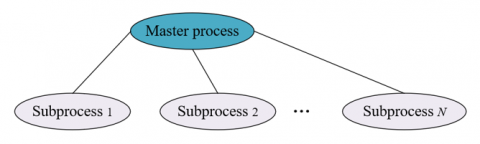
Despite progress in solving the inverse heat conduction problem using genetic algorithms and neural networks, these achievements have not yet been applied to solving the two-dimensional non-steady-state variable coefficient mathematical model, especially in the context of distributed solving with parallel genetic-neural network algorithms in high-speed local area network environments. This work represents the first integration of such parallel algorithms with the virtual boundary prediction method for the problem of service load balancing in cloud service environments. Specifically, a novel algorithm framework is developed, simulating the heat conduction process to predict and analyze server load distribution, and then utilizing an improved genetic-neural network algorithm to dynamically adjust server weights for load balancing. This algorithm achieves distributed computing on high-speed local area networks, significantly enhancing the efficiency of solution finding. Figure 1 presents the representation of the load balancing algorithm in the distributed computing model.
Figure 1. Representation of load balancing algorithm in a distributed computing model
Similar to the numerical computation of traditional heat transfer problems, a mathematical model for the server load issue, including control equations and boundary conditions, must first be established in this study. This model accounts for the dynamic changes in server load, analogous to the temperature distribution problem in heat conduction processes. In the design of thermal protection systems for aerospace vehicles, solving the characteristics of outer layer materials is a crucial step to ensure their normal operation and protection of internal structures under extreme temperatures. Originating from a Cartesian coordinate system, a two-dimensional heat conduction control equation is constructed to simulate the load heat distribution among multiple servers in cloud services. In this model depicted by the Cartesian coordinate system, "temperature" represents the server load level, while "heat flow" corresponds to the inflow and outflow of tasks. On this basis, corresponding boundary conditions are set, such as the maximum load capacity of servers and the arrival rate of service requests, to reflect the actual operation environment of cloud services. The two-dimensional heat conduction control equation and its boundary conditions are as follows:
$\frac{\partial i}{\partial s}=\frac{\partial}{\partial a}\left(j 1 \frac{\partial i}{\partial a}\right)+\frac{\partial}{\partial b}\left(j 2 \frac{\partial i}{\partial b}\right) 0<a, b<1, s>0$ (1)
Considering that the thermal conductivity of thermal protection system materials may vary across different layers in the thickness direction, the mathematical model is adjusted to allow for non-uniformity in thermal conductivity in the thickness direction, i.e., the model is adjusted to allow changes in thermal conductivity (representing the ease of load transfer between servers) in the "thickness direction" (analogous to load migration between servers). This implies that the rate of load transfer between servers can differ, possibly depending on the servers' configurations, network bandwidth, and other factors. Such adjustments permit the consideration that load migration between certain servers in actual cloud services might be more efficient than between others. The entire equation can thus be expressed as ∂i/∂s=∂/∂j(j∂i/∂a)+∂/∂b(j∂i/∂b) along with boundary conditions. Assuming temperature is represented by i, and the material's thermal conductivity is represented by j, this results in the following mathematical model:
$\left\{\begin{array}{l}\frac{\partial i}{\partial s}=\frac{\partial}{\partial a}\left(j \frac{\partial i}{\partial a}\right)+\frac{\partial}{\partial b}\left(k \frac{\partial i}{\partial b}\right) 0<a, b<1, s>0 \\ i(a, b, 0)=0 \\ i(0, b, s)=\operatorname{SIN}(2 \pi s) \operatorname{SIN}(\pi b) \\ i(1, b, s)=0, i(a, 0, s)=0, i(a, 1, s)=0 . s>0\end{array}\right.$ (2)
To accurately estimate the thermal conductivity characteristics of thermal protection materials, an objective function considering temperature errors was constructed in this study. This objective function evaluates the discrepancies between experimental data and numerical solutions, encompassing both measurement and model errors, that is, the deviation between predicted values based on service load and actual monitored values. The optimization of this objective function aims to minimize prediction errors, ensuring that load distribution closely matches actual demand, thereby optimizing the overall performance and resource usage efficiency of servers. Specifically, let j=j(a,i)=(X-a2)(Y-Zi+Fi2)+a2(R+Di+Hi2) from experience, where X, Y, Z, F, R, D, and H are unknown parameters, and let ϕ-=(X,Y,Z,F,R,D,H). Assuming the temperature history at a point o is represented by Sl(M,s), and the history of the calculated temperature value at that point is denoted by Sz. Clearly, there is a difference between Sl(su) and Sz(su). The following objective function expression is established:
$K(\bar{\varphi})=\|S l-S z\|^2=\frac{1}{V} \sum_{u=1}^V[S l(s u)-S z(s u, \bar{\varphi})]^2$ (3)
The entire problem is transformed into a nonlinear optimization problem, that is, under given constraints, the unknown parameters in the model (such as the position-dependent thermal conductivity) are adjusted to minimize the objective function. Using prior knowledge, upper and lower bounds that give X, Y, Z, F, R, D, and H practical significance are obtained, denoted as Xm, Xi, Ym, Yi, Zm, Zi, Fm, Fi, Rm, Ri, Dm, Di, Hm, and Hi, respectively. Thus, the original problem is transformed, with Xm≤X≤Xu, Ym≤Y≤Yi, Zm≤Z≤Zi, Fm≤F≤Fi, Rm≤R≤Ri, Dm≤D≤Di, and Hm≤H≤Hi serving as constraints.
In the context of designing thermal protection systems for aerospace vehicles, the inverse problem involves deducing the material's thermal conductivity from observed temperature data. Assuming the sought value of j is of the form: j=(1-a2)(0.1-0.01i+0.001i2)+a2(1.0+0.1i+0.01i2), then the objective function is I1=j(iaa+ibb)+ jaia+jbib, or i:=j(iaa+i)+H, where H=H(a,b,s)=jaia+jbib.
The function for thermal conductivity coefficient is derived to determine the direction of error reduction on the gradient. The updating method can adopt gradient descent or other optimization algorithms. The derivation results in ja=2x(0.9+0.1mi+0.009i2)+[(1-a2)(0.002i-0.01)+a2(0.1+0.02i)]ia, and jb=[(1-a2)(0.002i-0.01)+a2(0.1+0.02i)]ib. Further, let the time step be represented by ∇s and the spatial step by g, then the objective function is given by:
$(4+\vartheta) i_{u k}^{(b+1)}=i_{u-1, k}^{(b+1)}+i_{u+1, k}^{(b+1)}+i_{u, k-1}^{(b+1)}+i_{u, k+1}^{(b+1)}+f u k$ (4)
where, ϑ=g2/j∇sfk=ϑi(b)k+g2/jH, u,k=0,1,2,...,L, v=0,1,2,..., i(v)0k=SIN(2π(v))SIN(2πbk)i(v)Lk=0, and i(v)0k=0i(v)u0=0i(v)uL=0.
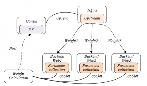
To enhance the performance status of web servers in providing cloud services on private cloud platforms, a web server cluster adaptive dynamic load balancing strategy for cloud services was designed and implemented. This strategy is based on the analogy of the heat conduction equation solution method for calculating the weight values of backend servers for the next cycle, as outlined in the previous section. The proposed strategy improves upon the existing Nginx weighted least connections algorithm by introducing a dynamic weight adjustment mechanism based on the heat conduction equation, thereby enhancing its adaptability. Given Nginx's widespread application in various web service scenarios and its capabilities for high concurrency handling and high configurability, the implementation of an adaptive load balancing strategy within this architecture has a solid practical foundation.
Figure 2. Implementation method of the adaptive dynamic load balancing strategy for cloud services
Specifically, this improved strategy takes the current number of connections and performance indicators of servers as "temperature" parameters, continuously monitoring and estimating each server's "temperature change", i.e., the trend of performance status change, through a numerical method akin to solving the heat conduction equation. Subsequently, server weights are dynamically adjusted according to these trends; servers with lower loads ("colder") receive higher weights, thus being more likely to accept new connection requests, while servers with higher loads ("hotter") have their weights reduced. Furthermore, backend servers periodically collect and report their performance parameters, such as Central Processing Unit (CPU) load, memory usage, and network bandwidth usage, to a central computing module. Employing an algorithm analogous to the heat conduction equation, this module predicts future performance trends of servers based on the collected performance parameters and calculates new weight values for each server accordingly. This process mimics the transfer of heat between materials, aiming to achieve an equilibrium distribution of server performance status. These weight values are then updated in the load balancer, which decides which server should receive new requests based on these weights, thus realizing task distribution based on the actual performance status of servers. Figure 2 presents the implementation method of the adaptive dynamic load balancing strategy for cloud services.
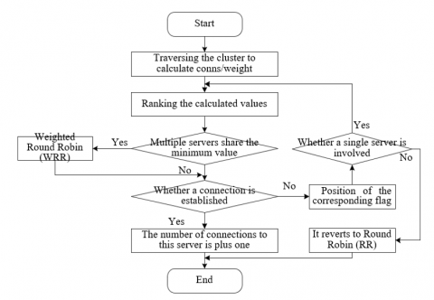
3.1 Improvements to the weighted least connections algorithm
The solution concept of the heat conduction equation has been applied to service load balancing optimization, particularly in improving the weighted least connections algorithm. In this enhanced algorithm, not only are the current connection numbers of backend servers considered, analogous to temperature, but server weights, analogous to heat capacity, are also introduced as adjusting factors. This equates to considering the "thermal efficiency" of each server in processing requests. When several servers exhibit the same ratio of connections to weight, the server with the largest weight, akin to the object with the highest heat capacity, is chosen to handle the next request. Moreover, the performance parameters of servers are updated periodically, influencing the dynamic adjustment of weights, similar to how temperature changes in an object affect the distribution of heat flow in heat conduction. Figure 3 displays the flowchart of the improved weighted least connections algorithm. Assuming the ratio of the target server's connection number to weight is represented by Z(Tl)/Q(Tl), and the minimum value obtained for this ratio is denoted by MIN{Z(Tu)/Q(Tu)}, the following is established:
$Z\left(T_l\right) / Q\left(T_l\right)=MIN\left\{Z\left(T_u\right) / Q\left(T_u\right)\right\}$ (5)
Figure 3. Flowchart of the improved weighted least connections algorithm
3.2 Weight calculation
The dynamic weight adjustment mechanism established in this study centers on the principle that the weights of backend servers are not statically set but are adjusted periodically based on the real-time load performance of the servers. Analogous to the redistribution of heat flow caused by temperature changes in an object during heat conduction, the performance parameters of servers, likened to temperature, are periodically evaluated and calculated to serve as the basis for weight adjustment. Just as heat tends to flow from high-temperature areas to low-temperature areas until thermal equilibrium is reached, the algorithm adjusts weights to allow servers that performed better (cooler) in the previous cycle to receive higher weights (larger "heat capacity") in the next cycle, taking on more connections, while servers with already high loads (hotter) see a reduction in their weights ("heat capacity" decreased), accepting fewer new requests. This dynamic adjustment strategy simulates the natural equilibrium process of heat conduction, enabling server clusters to adaptively adjust their load based on individual performance, thereby maintaining optimal overall system performance.
CPU idle rate, memory idle rate, and Input/Output (I/O) idle rate are selected as indicators of server load performance, and real-time data of these performance indicators are utilized to dynamically adjust server weights. This method is akin to considering the thermal conductivity of different materials in heat conduction, where the immediacy and accuracy of server performance indicator data act as key factors ensuring efficient heat transfer. To mitigate the transient performance deviations that periodic sampling might introduce, data are not merely collected at the end of cycle S but also at the midpoint S/2, and average values are calculated. This approach is similar to examining average temperature changes over a period rather than the temperature gradient at a single moment in heat conduction analysis. It helps to more accurately capture server performance changes, based on which weights are adjusted to ensure even load distribution. The selection of the length of period T is akin to determining an appropriate time step in heat conduction experiments; it should be neither too short, causing resource wastage due to frequent data collection, nor too long, preventing timely response to performance changes and leading to uneven load distribution. Assuming a backend server is represented by Tu, with weight denoted by D(Tu), CPU usage at moments S and S/2 represented by ZS and ZS/2, memory usage at moments S and S/2 by LS and LS/2, and I/O usage at moments S and S/2 by US and US/2, the following formula calculates the weight of each server:
$D\left(T_u\right)=O *\left(\begin{array}{c}J_{C P U} *\left(1-\frac{Z_{\frac{S}{2}}+Z_S}{2}\right) \\ +j_{M E M} *\left(1-\frac{L_{\frac{S}{2}}+L_S}{2}\right) \\ +j_{I O} *\left(1-\frac{U_{\frac{S}{2}}+U_S}{2}\right)\end{array}\right)$ (6)
The significance of CPU, memory, and I/O in performance, represented by jCPU, kMEM, and jIO, satisfies the following equation:
$j_{C P U}+j_{M E M}+j_{I O}=1$ (7)
3.3 Reference parameters and threshold values for weight change
The CPU and memory utilization rates of servers are considered key indicators representing the server load "temperature," analogous to the temperature of materials. When the CPU or memory utilization of a server increases to 80%, it is viewed as entering a "high temperature zone," capable of bearing less new load "heat." Consequently, the weight adjustment parameter for such servers is halved, effectively reducing their "heat capacity" and decreasing the number of requests they accept in the next cycle. Should the utilization further rise to 90%, it indicates that the server is "overheated" and in an overload state. At this point, the P value is adjusted to 0.1, significantly lowering the server's weight to prevent it from undertaking additional load. This is similar to reducing the heat flow input to areas of high heat concentration in the heat conduction process, ensuring a uniform and stable temperature distribution throughout the system. Since reaching an 80% utilization rate for I/O is relatively rare, adjustments for this within the model are not a primary consideration, though it remains a monitoring indicator for assessing the overall load situation of servers. The aforementioned scenarios can be expressed as follows:
$\left\{\begin{array}{l}\frac{Z_{\frac{S}{2}}+Z_S}{2}<0.8 A N D \frac{L_{\frac{S}{2}}+L_S}{2}<0.8 o=1 \\ \frac{Z_{\frac{S}{2}}+Z_S}{2} \geq 0.8 O R \frac{L_{\frac{S}{2}}+L_S}{2} \geq 0.8 o=0.5 \\ \frac{Z_{\frac{S}{2}}+Z_S}{2} \geq 0.9 O R \frac{L_{\frac{S}{2}}+L_S}{2} \geq 0.9 o=0.1\end{array}\right.$ (8)
To avoid overburdening the Nginx load balancer with frequent weight calculations, a concept of a threshold value, akin to the temperature gradient threshold in thermodynamic equilibrium, is introduced. Weight updates are conducted only when the change in server performance parameters exceeds this threshold, indicating a significant shift in the system's "temperature distribution." This is equivalent to considering heat exchange in the heat conduction process only when the temperature difference between objects surpasses a certain value, thus controlling the distribution of thermal energy to maintain system homeostasis. Weight remains unchanged when the absolute difference between the current cycle's D(Tu) and the previous cycle's DOL(Tu) is less than Z. Weight is updated only when the absolute difference exceeds Z. The formula for weight update is provided as follows:
$\left\{\begin{array}{l}\left|D_{O L}\left(T_u\right)-D\left(T_u\right)\right| \leq Z D_{N E}\left(T_u\right)=D_{O L}\left(T_u\right) \\ \left|D_{O L}\left(T_u\right)-D\left(T_u\right)\right|>Z D_{N E}\left(T_u\right)=D\left(T_u\right)\end{array}\right.$ (9)
3.4 Dynamic weight calculation for load balancers
A decimal weight value, D(Tu), reflecting the current load condition of the server, can be derived from the idle rates of the server's CPU, memory, and I/O. This weight value, analogous to the temperature gradient in heat conduction, indicates the trend and intensity of load energy flow among servers. A high idle rate for a server implies a lower "temperature," meaning it can bear more "heat energy," i.e., handle more requests. However, given that Nginx, serving as the load balancer, requires integer-form weight values, these decimal weight values must be converted into integer weights suitable for Nginx processing. This conversion process ensures the preservation of the relative proportions of weight values, thus maintaining the relative fairness and efficiency of load distribution among servers. The integer weight values q1,q2,…qv for the backend servers on the Nginx side are determined based on the proportion of each server's D(Tu), as follows:
$\left\{\begin{array}{l}q_1=\frac{D\left(T_1\right)}{\sum_{u=1}^v D\left(T_u\right)} * V \\ q_2=\frac{D\left(T_2\right)}{\sum_{u=1}^v D\left(T_u\right)} * V \\ \cdots \\ q_v=\frac{D\left(T_v\right)}{\sum_{u=1}^v D\left(T_u\right)} * V\end{array}\right.$ (10)
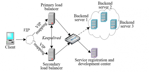
Figure 4. Network topology diagram of the load balancing test environment
This method ensures that even in the process of weight value discretization, requests can be dynamically and reasonably distributed to each server based on real-time changes in server performance parameters, leading to a more balanced server load and thus optimizing the performance of the entire cloud service system. Figure 4 provides the network topology diagram of the load balancing test environment.
The results of solving the heat conduction equation, as presented in Table 1, compare three different methods: the back propagation (BP) neural network, genetic algorithm, and the method proposed in this study, which combines the genetic algorithm and neural network. The identification values derived from each method were compared with actual values, using absolute and relative errors as metrics to assess the accuracy of the models. For the parameter X, the method proposed in this study exhibited the smallest relative error at 1.48%, compared to 2.63% and 1.89% for the BP neural network and genetic algorithm, respectively. This indicates the proposed method's superior accuracy in estimating parameter X. In terms of parameters Y, Z, F, R, D, and H, the proposed method also demonstrated lower relative errors, indicating better overall precision. It can be concluded that the method integrating the genetic algorithm and neural network, as proposed in this study, predicts thermal physical parameters more accurately in solving the inverse problem of the two-dimensional nonlinear heat conduction equation, compared to using the BP neural network or genetic algorithm alone. The effectiveness of the proposed method is evidenced by the smallest absolute and relative errors in the identification values of all parameters, illustrating higher accuracy and reliability in parameter estimation.
Table 1. Comparative results of solving the heat conduction equation
|
Parameter |
X |
Y |
Z |
F |
R |
D |
H |
|
|
Actual value |
1.0 |
0.1 |
0.01 |
0.001 |
1.0 |
0.1 |
0.01 |
|
|
BP neural network |
Identification value |
0.9652 |
0.11245 |
0.00948 |
0.00098 |
1.1245 |
0.09456 |
0.00912 |
|
Absolute error |
0.0265 |
0.00312 |
0.00048 |
0.00009 |
0.02856 |
0.00421 |
0.00077 |
|
|
Relative error (%) |
2.63 |
3.12 |
4.78 |
9.01 |
2.89 |
4.26 |
7.78 |
|
|
Genetic algorithm |
Identification value |
1.0156 |
0.0978 |
0.0097 |
0.00093 |
0.9785 |
0.1147 |
0.00935 |
|
Absolute error |
0.0187 |
0.0017 |
0.0002 |
0.00006 |
0.0125 |
0.0031 |
0.00052 |
|
|
Relative error (%) |
1.89 |
1.78 |
2.01 |
3.12 |
1.34 |
3.21 |
5.21 |
|
|
Proposed method |
Identification value |
1.02356 |
0.09785 |
0.01126 |
0.00095 |
0.98542 |
0.11256 |
0.00945 |
|
Absolute error |
0.01452 |
0.00156 |
0.00025 |
0.00005 |
0.02154 |
0.00336 |
0.00044 |
|
|
Relative error (%) |
1.48 |
1.65 |
2.56 |
5.1 |
2.15 |
3.38 |
4.45 |
|
Table 2. Relationship between the number of computer nodes and running time
|
Number of Computer Nodes |
1 |
2 |
3 |
4 |
5 |
|
Running time (seconds) |
2356.658 |
1635.124 |
987.235 |
825.648 |
759.361 |
|
Number of Computer Nodes |
6 |
7 |
8 |
9 |
10 |
|
Running time (seconds) |
712.365 |
689.214 |
785.124 |
821.236 |
934.586 |
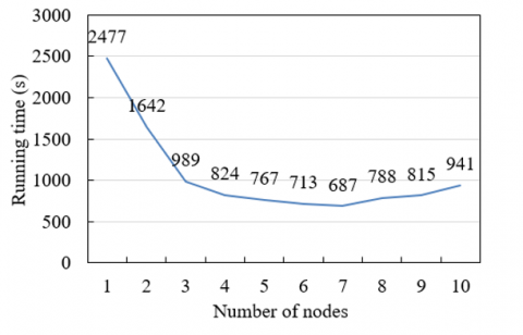
Figure 5. Relationship between the number of computer nodes and running time
Table 2 illustrates the impact of increasing the number of computer nodes on the running time of the method proposed. It is observed from the table that, as the number of computer nodes increases, the overall running time tends to decrease, although not linearly. Specifically, when the number of nodes increases from 1 to 5, the running time significantly reduces from 2356.658 seconds to 759.361 seconds. This indicates that the completion time of tasks can be significantly reduced with the addition of more computing resources, aligning with the fundamental principles of parallel computing. However, as the number of nodes continues to increase, the reduction in running time begins to diminish, and even increases when moving from 7 to 8 computer nodes, due to the influence of communication overhead and the management costs of task distribution. The minimum running time of 689.214 seconds is reached with 7 computer nodes, after which an increase in node count results in increased running time. It can be concluded that the model proposed in this study effectively utilizes parallel computing resources to reduce running time, as clearly demonstrated in the data from one to five nodes.
Figure 5 depicts how the running time of the proposed method changes with the increase in the number of computer nodes. As the number of nodes increases from 1 to 7, the running time decreases from 2477 seconds to 687 seconds, indicating that parallel processing can significantly reduce computation time. However, when the number of nodes increases to 8, the running time paradoxically rises to 788 seconds, and as the number of nodes continues to increase to 10, the running time remains at a higher level (815 seconds and 941 seconds). This is due to the fact that beyond a certain point, the overhead of network communication and task coordination exceeds the time savings brought by parallel computing. It can be concluded that the model proposed in this study effectively leverages parallel computing resources, as evident from the significant decrease in running time when increasing the node count from 1 to 7. This indicates that the model is well-designed for parallelization, effectively distributing computing tasks across multiple processing nodes.
Table 3 provides parallel computing performance data for two methods: the traditional genetic algorithm and the method proposed in this study, which integrates the genetic algorithm and neural network. This data includes the parallel speedup ratio and efficiency as the number of computer nodes increases for both methods. Analyzing these metrics helps understand the parallel performance of the models. Data from Table 3 show that for the traditional genetic algorithm, the speedup ratio increases with the number of nodes but begins to decline starting from seven nodes, indicating a weakening of parallelization effects beyond a certain level of node increase. Conversely, the parallel speedup ratio of the method proposed in this study generally increases with the number of nodes, although it also declines after eight nodes. However, the magnitude of this decline is less than that of the traditional genetic algorithm, and it remains constant at nine nodes, indicating maintained performance at higher levels of parallelism. The parallel efficiency of the traditional genetic algorithm shows a clear downward trend as the number of nodes increases, whereas the parallel efficiency of the method proposed in this study, although also decreasing with more nodes, maintains a higher level overall. Notably, at three nodes, it reaches an efficiency of 0.815, meaning a more than 2.5 times speed increase with a threefold increase in computing resources. In summary, the model combining the genetic algorithm and neural network demonstrates superior performance in parallel computing compared to the traditional genetic algorithm, especially in maintaining high parallel efficiency and speedup ratio. This indicates that the proposed method can more effectively utilize increased computing resources to enhance computation speed and reduce computation time.
Table 3. Speedup ratio and parallel efficiency
|
Number of Computer Nodes |
2 |
3 |
4 |
5 |
6 |
7 |
8 |
9 |
10 |
|
|
Genetic algorithm |
Parallel speedup ratio |
1.53 |
2.23 |
2.78 |
3.21 |
3.12 |
3.45 |
2.89 |
2.31 |
2.24 |
|
Parallel efficiency |
0.758 |
0.715 |
0.712 |
0.624 |
0.524 |
0.512 |
0.356 |
0.256 |
0.214 |
|
|
Proposed method |
Parallel speedup ratio |
1.4562 |
2.365 |
2.895 |
3.125 |
3.215 |
3.456 |
3.124 |
3.124 |
2.564 |
|
Parallel efficiency |
0.745 |
0.815 |
0.723 |
0.635 |
0.556 |
0.519 |
0.378 |
0.325 |
0.256 |
|
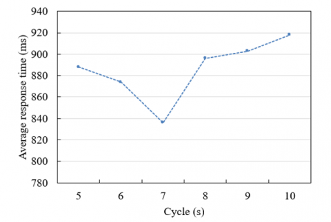
Figure 6. Line graph of the relationship between average response time and cycle T
Figure 6 shows the change in the system's average response time as cycle T increases. It is observed that between cycles 5 and 7, the average response time decreases from 888 milliseconds to 836 milliseconds. This indicates an improvement in the system's response time as the cycle increases, due to the effective distribution of requests by the adaptive dynamic load balancing strategy proposed in this study, thereby reducing response time. However, from cycle 7 to cycle 10, the average response time gradually increases, from 836 milliseconds to 918 milliseconds. This trend suggests that beyond a certain cycle length, the average response time increases due to the influence of the load distribution strategy. This is attributed to the system needing to handle more requests before re-evaluating and adjusting server weights over longer cycles, leading to resource overload or imbalance in the short term. It can be concluded that the algorithm proposed in this study effectively reduces average response time in the initial phase (i.e., as T increases from 5 to 7), demonstrating the algorithm's effectiveness in reflecting and adjusting to real-time loads. This emphasizes the algorithm's ability to adapt promptly in the face of dynamic load changes, thereby optimizing performance. As the cycle continues to increase, system performance begins to decline, highlighting some limitations in the load distribution of the algorithm or the improper setting of cycle lengths. Excessively long cycles lead to untimely adjustments; therefore, in practical applications, the cycle length needs to be optimized based on system load characteristics to ensure that the response time remains within an ideal range.
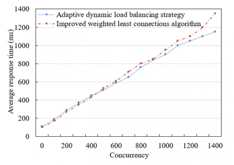
Figure 7. Line graph illustrating the relationship between average response time and concurrency
Figure 7 displays the changes in average response time under different levels of concurrency for the adaptive dynamic load balancing strategy and the improved weighted least connections algorithm proposed in this study. At lower levels of concurrency (0 to 400), the response time trends of both algorithms are similar, and the values are close, indicating that under light load conditions, both algorithms can effectively handle requests with little difference in response time. As the concurrency continues to increase (400 to 1000), the increase in average response time for the adaptive dynamic load balancing strategy is less than that for the improved weighted least connections algorithm. For example, at a concurrency of 1000, the response time for the adaptive strategy is 510 milliseconds, compared to 530 milliseconds for the improved weighted least connections algorithm. This demonstrates the advantage of the adaptive strategy under moderate load conditions. At higher levels of concurrency, especially above 1400, the response time for the adaptive strategy is over 150 milliseconds lower than that for the improved weighted least connections algorithm. This gap illustrates that under high load conditions, the adaptive strategy can more effectively distribute the load, maintaining lower response time. The algorithm proposed in this study shows good performance under different load conditions, especially in maintaining low latency under high concurrency situations, thereby enhancing user experience.
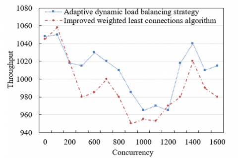
Figure 8. Line graph of the relationship between throughput and concurrency
Figure 8 illustrates the throughput of the adaptive dynamic load balancing strategy and the improved weighted least connections algorithm under various levels of concurrency. It is observed that at low concurrency levels (0 to 200), the throughput of both algorithms is nearly identical, with the adaptive dynamic load balancing strategy even showing slightly lower throughput at zero concurrency. This indicates that under low load conditions, both algorithms are capable of efficiently handling requests with comparable performance. As the concurrency increases to 600 and 800, the throughput of both algorithms decreases, but the adaptive dynamic load balancing strategy exhibits less reduction, demonstrating better stability. When concurrency further increases to between 1000 and 1400, the throughput of the adaptive dynamic load balancing strategy shows better stability and a slight increase, while the throughput of the improved weighted least connections algorithm first declines and then stabilizes. Notably, at a concurrency of 1400, the throughput of the adaptive strategy is approximately 30 higher than that of the improved algorithm. With a further increase in concurrency to 1600, the throughput of the adaptive dynamic load balancing strategy decreases but remains above 965, whereas the throughput of the improved weighted least connections algorithm drops to around 950. It can be concluded that the adaptive dynamic load balancing strategy maintains comparable performance to the improved weighted least connections algorithm at low to medium concurrency levels, and exhibits better stability and efficiency at high concurrency levels. Facing a large number of concurrent requests, the proposed algorithm maintains a higher throughput, reflecting its excellent adaptive capability and effective management of load fluctuations.
The article initially introduces a novel model that combines the genetic algorithm and neural network to solve the inverse problem of the two-dimensional nonlinear heat conduction equation, namely predicting thermal physical parameters through observational data. The innovation of this method lies in leveraging the global search capability of the genetic algorithm and the powerful fitting ability of the neural network to achieve high-accuracy solutions for complex heat conduction problems. Building on the first part, an adaptive dynamic load balancing strategy algorithm is proposed. By applying the solution of the heat conduction equation to calculate the weights of backend servers, this method optimizes and improves the weighted least connections algorithm in Nginx, achieving the objective of dynamically adjusting server weights based on real-time load. This offers a new solution for load balancing in web server clusters within cloud services.
The article compares the results of solving the heat conduction equation with the proposed model, verifying its accuracy. The relationship between the number of computer nodes and running time is discussed, and the model's computational performance is studied by comparing speedup ratios and parallel efficiencies. Line graphs illustrating the relationship between average response time and cycle T, average response time and concurrency, and throughput and concurrency are drawn, comparing and analyzing the performance of different load balancing strategies.
Future research will further optimize the model combining the genetic algorithm and neural network, enhancing its solution accuracy and speed in more complex situations. The application of the proposed model and algorithm to the solution of other types of partial differential equations, as well as optimization problems in other fields, will be explored.
[1] Hemam, S.M., Hioual, O., Hioual, O. (2023). Dynamic load balancing upon the replication and deletion of cloud services. Journal of Intelligent & Fuzzy Systems, 44(1): 381-393. https://doi.org/10.3233/JIFS-221989
[2] Chanyour, T., Malki, M.O.C. (2021). Deployment and Migration of virtualized services with joint optimization of backhaul bandwidth and load balancing in mobile edge-cloud environments. International Journal of Advanced Computer Science and Applications, 12(3): 566-576. https://doi.org/10.14569/IJACSA.2021.0120368
[3] Dornala, R.R. (2023). An advanced multi-model cloud services using load balancing algorithms. In 2023 5th International Conference on Inventive Research in Computing Applications, pp. 1065-1071. https://doi.org/10.1109/ICIRCA57980.2023.10220892
[4] Saba, T., Rehman, A., Haseeb, K., Alam, T., Jeon, G. (2023). Cloud-edge load balancing distributed protocol for IoE services using swarm intelligence. Cluster Computing, 26(5): 2921-2931. https://doi.org/10.1007/s10586-022-03916-5
[5] Mohammadian, V., Navimipour, N.J., Hosseinzadeh, M., Darwesh, A. (2023). LBAA: A novel load balancing mechanism in cloud environments using ant colony optimization and artificial bee colony algorithms. International Journal of Communication Systems, 36(9): e5481. https://doi.org/10.1002/dac.5481
[6] Halappa, A., Rajesh, A. (2023). Performance analysis of load balancing mechanism in cloud computing. In 2023 International Conference on Applied Intelligence and Sustainable Computing, Dharwad, India, pp. 1-5. https://doi.org/10.1109/ICAISC58445.2023.10199269
[7] Choubey, P., Mohapatra, B. (2022). Comparative analysis of load balancing algorithm in cloud computing. In International Conference on Signal Processing and Integrated Networks, Noida, India, pp. 187-199. https://doi.org/10.1007/978-981-99-1312-1_15
[8] Ramya, K., Ayothi, S. (2023). Hybrid dingo and whale optimization algorithm-based optimal load balancing for cloud computing environment. Transactions on Emerging Telecommunications Technologies, 34(5): e4760. https://doi.org/10.1002/ett.4760
[9] Zhang, Y., Jia, Y., Lin, Y. (2023). A new multiscale algorithm for solving the heat conduction equation. Alexandria Engineering Journal, 77: 283-291. https://doi.org/10.1016/j.aej.2023.06.066
[10] He, H., Zhang, X. (2024). A general numerical method for solving the three-dimensional hyperbolic heat conduction equation on unstructured grids. Computers & Mathematics with Applications, 158: 85-94. https://doi.org/10.1016/j.camwa.2024.01.012
[11] Saleh, M., Kovács, E., Kallur, N. (2023). Adaptive step size controllers based on Runge-Kutta and linear-neighbor methods for solving the non-stationary heat conduction equation. Networks and Heterogeneous Media, 18(3): 1059-1082. https://doi.org/10.3934/nhm.2023046
[12] Shevelev, V.V. (2023). The method of integral transformations for solving boundary-value problems for the heat conduction equation in limited areas containing a moving boundary. Journal of Engineering Physics and Thermophysics, 96(1): 168-177. https://doi.org/10.1007/s10891-023-02673-5
[13] Al-Nuaimi, B.T., Al-Mahdawi, H.K., Albadran, Z., Alkattan, H., Abotaleb, M., El-kenawy, E.S.M. (2023). Solving of the inverse boundary value problem for the heat conduction equation in two intervals of time. Algorithms, 16(1): 33. https://doi.org/10.3390/a16010033
[14] Yang, Z., Wang, Y., Huang, Z., Rao, Z. (2021). Characteristic analysis of a new high-static-low-dynamic stiffness vibration isolator based on the buckling circular plate. Journal of Low Frequency Noise, Vibration and Active Control, 40(3): 1526-1539. https://doi.org/10.1177/1461348420904864
[15] Huang, M.F., Tu, Z., Li, Q., Lou, W., Li, Q.S. (2017). Dynamic wind load combination for a tall building based on copula functions. International Journal of Structural Stability and Dynamics, 17(8): 1750092. https://doi.org/10.1142/S0219455417500924
[16] Chi, X., Yao, J., Yu, H. (2018). A hybrid load balance method using evolutionary computing. In Proceedings of the Australasian Joint Conference on Artificial Intelligence-Workshops, Wellington, New Zealand, pp. 15-19. https://doi.org/10.1145/3314487.3314490
[17] Lifflander, J., Slattengren, N.L., Pébaÿ, P.P., Miller, P., Rizzi, F., Bettencourt, M.T. (2021). Optimizing Distributed Load Balancing for Workloads with Time-Varying Imbalance. In 2021 IEEE International Conference on Cluster Computing, Portland, OR, USA, pp. 238-249. https://doi.org/10.1109/Cluster48925.2021.00039
[18] Lin, Z., Liu, X., Zhou, H., Wu, J. (2022). Adaptive time-varying routing for energy saving and load balancing in wireless body area networks. IEEE Transactions on Mobile Computing, 23(1): 90-101. https://doi.org/10.1109/TMC.2022.3213471
[19] Xu, X., Zhao, N., Wang, L., Yao, X., Zhou, L. (2023). Research on time-varying dynamic response aggregation model of distributed generator participating in active distribution network. Energy Reports, 9: 1546-1556. https://doi.org/10.1016/j.egyr.2023.04.159
[20] Karpeev, A. (2022). Dynamic load balancing algorithm for continuum mechanics problems with essential redistribution of workloads among the processes. Journal of Physics: Conference Series, 2154(1): 012007. https://doi.org/10.1088/1742-6596/2154/1/012007
[21] Wang, F., Yao, H., Zhang, Q., Wang, J., Gao, R., Guo, D., Guizani, M. (2021). Dynamic distributed multi-path aided load balancing for optical data center networks. IEEE Transactions on Network and Service Management, 19(2): 991-1005. https://doi.org/10.1109/TNSM.2021.3125307
[22] Zhu, A., Chang, Q., Xu, J., Ge, W. (2023). A dynamic load balancing algorithm for CFD–DEM simulation with CPU–GPU heterogeneous computing. Powder Technology, 428: 118782. https://doi.org/10.1016/j.powtec.2023.118782
[23] Mouawad, M., Mah, F., Dziong, Z. (2022). RRH-Sector selection and load balancing based on MDP and dynamic RRH-Sector-BBU mapping in C-RAN. Computer Networks, 215: 109192. https://doi.org/10.1016/j.comnet.2022.109192