Shuang Huang*![]() | Dan Huang
| Dan Huang![]()
© 2023 IIETA. This article is published by IIETA and is licensed under the CC BY 4.0 license (http://creativecommons.org/licenses/by/4.0/).
OPEN ACCESS
In the realm of global manufacturing, the proliferation of Laser Powder Bed Fusion (LPBF) technologies has necessitated an in-depth understanding of the dynamics between thermal flow and stress fields during its operative procedures. Interactions between these fields have been observed to induce thermal distortions in components, potentially jeopardizing the structural integrity and operational efficiency of the end products. Insights have been garnered through conventional finite element methods and empirical models, yet these methodologies encounter evident constraints when deciphering highly nonlinear, multi-scale systems. This research delves into the employment of deep learning techniques for the cooperative modelling of the aforementioned fields, suggesting an innovative approach to thermal distortion predictions. The outcomes derived from this inquiry are foreseen to unveil novel optimization strategies for laser melting manufacturing methodologies, propelling the evolution of this specialized field.
Laser Powder Bed Fusion (LPBF), thermal flow, stress field, deep learning, thermal distortion prediction
In the global manufacturing landscape, the boundaries of production speed, accuracy, and potential are being continuously redefined by the advent of LPBF technologies [1-5]. This form of additive manufacturing facilitates the production of intricate components, which, owing to their high precision, customization, and geometric complexity, were previously unattainable with traditional manufacturing techniques [6, 7]. However, the evolution of this innovative approach has not been without its challenges. A significant hurdle has been identified in the interactions between thermal flow and stress fields during the laser melting process. Such interactions have been linked to the onset of thermal distortions in components, potentially diminishing the integrity and efficiency of the final product [8-10].
Addressing these challenges holds broader implications than merely refining component quality. A deeper comprehension of these field interactions, it is believed, could usher in expansive optimization opportunities for the overarching production cycle, leading towards more streamlined and cost-effective manufacturing [11, 12]. Among the tools to achieve this, deep learning, at the forefront of modern artificial intelligence techniques, has been heralded for its capabilities in encapsulating and simulating these multifaceted relations [13-15].
While valuable perspectives on the interaction dynamics between thermal flow and stress fields have been offered by finite element methods and empirical models, these techniques exhibit discernible limitations [16, 17]. Confronted with highly nonlinear, multi-scale systems, the aforementioned methods can sometimes underperform [18-20]. Thus, the call for a renewed methodology that aptly captures the interplay between thermal flow and stress fields has grown louder.
In response to this, a thorough investigation into the construction of dual-field models within the LPBF domain was undertaken. Emphasis was laid on studying both laminar and turbulent flow models concerning fluid dynamics and heat transfer within the melt pool. Notably, a pioneering strategy for predicting product thermal distortions, underpinned by feature extraction from these fields, was introduced. By treating the combined features of the thermal flow and stress domains as cooperative inputs, a groundbreaking approach to predict product thermal distortion levels was formulated. The revelations from this inquiry are not merely poised to foster innovative solutions for challenges inherent to LPBF but also to set the groundwork for emergent breakthroughs in the broader additive manufacturing sphere.
2.1 Model establishment
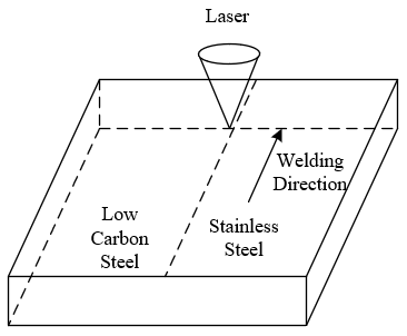
Laser Powder Bed Fusion (LPBF), also known as Direct Metal Laser Sintering (DMLS), represents a technique within additive manufacturing, encompassing several interconnected physical processes. When laser beams irradiate the surface of metal powders, the metal absorbs the laser energy and undergoes rapid heating, resulting in localized melting. This induces a prominent temperature gradient, culminating in the formation of a melt pool. Metals, under elevated temperatures, undergo a phase transition from solid to liquid, manifesting as this melt pool. Due to surface tension, variations in the depth and width of the melt pool, and uneven temperatures, pronounced flows are observed within the melt pool. Heat from the melt pool is conducted to the surrounding solid metal, instigating movements at the solid-liquid interface and accompanying phase transitions such as solidification, undercooling, and recrystallisation. Figure 1 presents a schematic diagram of the melting manufacturing process.
Figure 1. The LPBF process
Owing to the high-energy density and brief thermal input of LPBF, metals undergo a rapid cooling process. Such swift cooling generates thermal stresses within the metal, especially at interfaces where the melt pool solidifies. As metals cool from a liquid to a solid state, volume changes occur, leading to the genesis of phase transformation stresses. If these thermal stresses surpass the material's yield strength, thermal cracking can ensue. Additionally, residual stresses arising from non-uniform cooling and solidification may also result in thermal distortions of the components.
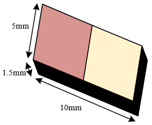
In the LPBF process, constructing models for the thermal flow and stress fields becomes crucial for accurate prediction and optimization. For precise simulation of these fields, grid partitioning strategy emerges as pivotal. Given that the melt pool area is where thermal flow and stress variations are most intense, higher grid resolutions are necessitated. In this study, a dense tetrahedral or hexahedral grid was chosen in this region to capture the dynamic behaviour of the melt pool and the phase transition process. Figure 2 illustrates the grid partitioning strategy.
Figure 2. Strategy of grid partitioning
When constructing thermal and stress field models for the LPBF process, a set of assumptions typically must be established to simplify real-world problems, ensuring that mathematical models can be effectively applied under actual conditions. Core assumptions, grounded in the study's research content and objectives, include:
(1) Steady state and unsteady state assumption
Interaction between the laser and the material is instantaneous, and the formation and flow of the melt pool are dynamic. A steady-state (transient) assumption is often adopted, meaning that in the model, time is considered a variable.
(2) Continuum medium assumption
Although the material consists of tiny particles, at this scale, the material is assumed to be a continuous medium, meaning that the specific shape and size of the powder particles aren't taken into account, focusing only on their macroscopic behaviour.
(3) Isotropic material assumption
It is assumed that the properties of the material (such as thermal conductivity or elastic modulus) are consistent in all directions. This simplifies the model, yet relatively accurate results can still be obtained.
(4) Temperature-independent parameters
Some properties of the material (like thermal conductivity or viscosity) are considered constant and not dependent on temperature. However, more precise models may consider the temperature-dependence of these parameters.
Characteristics of thermal and stress fields during the welding process are influenced by the solid phase, liquid phase, and solid-liquid mixture phase. The solid phase, typically distant from the centre of the melt pool, is in a relative thermal equilibrium. In this region, heat is mainly transmitted by conduction, resulting in smaller temperature gradients. Residual stress is produced due to thermal expansion and contraction caused by welding. As the distance from the melt pool increases, residual stresses gradually decrease. The liquid phase, being the central part of the melt pool, has the highest temperature. In this zone, in addition to conduction, convection also plays a significant role in heat transfer. The flow of molten metal carries heat, leading to complex temperature distributions. In the liquid phase, since the material is in a liquid state, stress generation is minimal. However, at the interface between liquid and solid, stress concentration may occur due to differing thermal expansion coefficients. The solid-liquid mixture phase is the transition zone between the solid and liquid phases and is the most complex area. Here, some materials are in the solid state while others are in the liquid state. Both conduction and convection are involved in heat transfer, and the solid-liquid interface dynamically changes, making the thermal field intricate. In the solid-liquid mixture zone, volume shrinkage due to the solidification of molten metal and thermal expansion of solid metal occur concurrently, potentially leading to stress concentration and thermal cracking. Additionally, rapid cooling and thermal expansion in localized areas due to the dynamic change of the solid-liquid interface may generate significant stresses.
The solid-liquid interface during the welding process dynamically changes, and accurately tracking and simulating this interface demands substantial computational resources. In this study, the solid-liquid zone is regarded as a porous medium, and the degree of solid-liquid mixing is described by "porosity." An approach facilitating the handling of the complexity of the solid-liquid mixture zone during the welding process. An infinitesimally small number, represented by $\gamma$, is assumed to avoid a denominator of zero. The fuzzy zone constant is represented by SMU, and the volume fraction of the liquid is denoted by $\alpha$. This method can be implemented by adding the following source terms to the momentum equation:
$A_z=i \frac{(1-\alpha)^2}{\alpha^3+\gamma} S_{M U}$ (1)
$A_t=c \frac{(1-\alpha)^2}{\alpha^3+\gamma} S_{M U}$ (2)
$A_x=q \frac{(1-\alpha)^2}{\alpha^3+\gamma} S_{M U}$ (3)
Assuming the solid phase line temperature and liquid phase line temperature are represented by Ya and Yy respectively, the liquid volume fraction α is determined by:
$\alpha=\left\{\begin{array}{l}0, Y<Y_a \\ 1, Y>Y_m \\ \left(Y-Y_a\right) /\left(Y_m-Y_a\right), Y_a<Y<Y_m\end{array}\right.$ (4)
From the analysis, it is understood that buoyancy, vapour pressure produced by the evaporation of liquid metal, and surface tension play crucial roles in the dynamics of the melt pool and the welding outcome. Convection flows caused by buoyancy can alter the heat flow distribution, thereby affecting the cooling rate and temperature distribution in the welding area. Backpressure affects the surface of the melt pool and can lead to its unstable oscillations or splashing. Surface tension causes the melt pool to minimize its surface area, forming a specific melt pool shape. The combined effect of these factors influences the outcome of the welding process, such as the melt pool shape and the quality of the weld seam. Incorporating all these factors can enhance the accuracy of the model.
2.2 Turbulence equations and boundary conditions
During the LPBF process, the intense heat flux density generated by the laser on the workpiece results in vigorous motion within the melt pool, likely transforming into turbulence. Turbulence enhances fluid mixing, thereby amplifying heat transfer effects. For laser welding, this intensified heat transfer effect can lead to changes in the depth and shape of the melt pool, subsequently influencing the formation and quality of the weld seam. To address the impact of turbulence on flow and heat transfer in the melt pool, the $R N G_{k-\varepsilon}$ turbulence model is employed for simulation calculations. If turbulent energy is denoted by j and the turbulent diffusivity is represented by $\gamma$, then the expressions for turbulent energy are:
$\frac{\partial(\vartheta \gamma)}{\partial y}+\frac{\partial\left(\vartheta \gamma i_u\right)}{\partial z_u}=\frac{\partial}{\partial z_k}\left(\alpha_\gamma F \frac{\partial j}{\partial z_u}\right)+H_j+\vartheta \gamma$ (5)
$\frac{\partial(\vartheta \gamma)}{\partial y}+\frac{\partial\left(\vartheta \gamma i_u\right)}{\partial z_u}=\frac{\partial}{\partial z_k}\left(\alpha_\gamma F \frac{\partial \gamma}{\partial z_u}\right)+\frac{H_{1 \gamma}^*}{j} H_j-V_{2 \gamma} \vartheta \frac{\gamma^2}{j}$ (6)
Due to the high power density and focused characteristics of lasers, significant temperature gradients arise in the melt pool during the laser welding process. Such pronounced temperature gradients on the melt pool surface lead to a marked surface tension gradient, resulting in Marangoni convection. It is observed that Marangoni convection alters the flow patterns within the melt pool, subsequently affecting the shape and size of the pool. Direct consequences of these alterations are witnessed in the width and depth of the weld bead. Moreover, an upward movement in the centre of the melt pool and a downward shift at its edges due to Marangoni convection can increase the depth of the melt pool, impacting the welding penetration depth. Assuming the reference temperature is represented by Y0 and the surface tension temperature gradient coefficient by Sa, the calculation formula for melt pool surface tension is given by:
$\varepsilon=\varepsilon_o+S_a\left(Y-Y_p\right)$ (7)
It is assumed that the laser power is denoted by O, the radius of the laser heat source by s=n=e, and the depth of the heat source by f. When considering a welding heat source with a Gaussian distribution volumetric heat source, its expression is described by:
$\begin{aligned} & W(z, t, x, y)=\frac{3 O}{\tau s n f} \exp \left(-\frac{3\left(z-z_0-C_q y\right)^2}{s^2}\right) \\ & \exp \left(-\frac{3 t^2}{n^2}\right) \exp \left(-\frac{3 x^2}{f^2}\right)\end{aligned}$ (8)
During the LPBF process, considerable heat is generated in the melt pool due to the interaction between the laser beam and the workpiece material. However, not all the heat contributes to melting the material. A portion of this heat is lost from the melt pool in the form of convection and radiation. To accurately describe and predict the outcomes of the laser melting process, these heat losses need to be taken into account. Convective heat losses primarily occur at the surface of the melt pool, involving interactions between the liquid metal and surrounding gases, such as protective gases. When an object's temperature exceeds that of its surrounding environment, heat is released in the form of radiation. In high-temperature melt pools, radiative heat loss can be notably significant. Assuming the Boltzmann constant is represented by $\delta_n$, the emissivity by γn, and the ambient temperature by Ys, then the calculation formula for heat losses due to convection and radiation is:
$w_{L O}=g_v\left(Y-Y_s\right)+\delta_n \gamma_n\left(Y^4-Y_s^4\right)$ (9)
During the LPBF process, thermal distortion emerges as a complex multifactorial procedure influenced by various parameters. To forecast thermal distortion, features related to this process must be clearly defined. Firstly, definitions are given for thermal field indicators, stress field indicators, laser melting manufacturing condition indicators, and product shape indicators.
Indicators of thermal field characteristics include: (1) Maximum temperature, referring to the highest temperature within the melt pool; (2) Temperature gradient, indicating the difference between temperatures inside and outside the melt pool; (3) Cooling rate, which is the speed at which the material cools from a molten to a solidified state; (4) Melt pool depth-to-width ratio, influencing the shape and flow characteristics of the melt pool. Theses parameters determine the heating and cooling characteristics of the material, subsequently influencing the dynamics, solidification rate, and geometry of the melt pool. Indicators of stress field characteristics include: (1) Maximum stress, which is the highest stress value generated from thermal expansion and contraction; (2) Stress gradient, highlighting the difference in stress within and around the weld seam; (3) Residual stress, referring to the internal stress remaining after the material cools; (4) Degree of plastic deformation, defining the extent of material deformation at high temperatures. These parameters describe the stress state in and around the welding zone. Due to the uneven distribution of temperature, different parts of the melt pool undergo varying expansions and contractions, leading to the accumulation of stress and plastic deformation. The features from these two categories are represented byφ={φ1,φ2,...,φN} and ψ={ψ1,ψ2,...,ψB}, where the value of the u-th feature is indicated by ψu. ψu consists of Bu position points and can be described as ψu={ψu1,ψu2,...,ψuBu}, with the k-th point on the u-th feature denoted by ψuk.
Indicators of LPBF conditions include: (1) Laser power, or the power setting of the laser beam; (2) Laser scanning speed, or the speed at which the laser beam moves across the workpiece surface; (3) Focal length, the distance between the laser focal point and the workpiece surface; (4) Shielding gas velocity and type, namely the velocity and type of the gas used to protect against oxidation and other adverse chemical reactions. These conditions directly influence the formation of the melt pool, heat input, and heat distribution, thereby affecting material melting, solidification, and generation of thermal stresses. This category of features is denoted by $\zeta=\left\{\zeta_1, \zeta_2, \ldots, \zeta_{B^* L}\right\}$, with the total number of conditions represented by B*L.
Indicators of product shape include: (1) Product thickness, indicating the thickness of the workpiece, affecting heat transfer and cooling rate; (2) Welding length, referring to the total length of the weld seam; (3) Weld seam width, related to the diameter and shape of the laser beam; (4) Welding direction, such as sequential or alternating welding. The shape and dimensions of the workpiece influence the method and speed of heat transfer, consequently affecting temperature distribution and melt pool behaviour. Features of this category are expressed by ψ={ψ1,ψ2,...,ψL}, with the function on the m-th direction denoted by Om and the shape image represented by ψomu. The process of obtaining the product shape coding from the autoencoder is given by equations below:
$\begin{aligned} & \psi o_{m u}=O_m\left(\psi_u\right), m=1,2, \ldots, 6 \\ & \xi h_u=N E_h\left(\psi o_{1 u}, \psi o_{2 u}, \psi o_{3 u}, \psi o_{4 u}, \psi o_{5 u}, \psi o_{6 u}\right)\end{aligned}$ (10)
Local geometric features near a point on the product appearance are represented by $\xi=\left\{\xi m_u{ }^1, \xi m_u{ }^2, \ldots, \xi m_u{ }^{B u}\right\}$. The normal vector, maximum principal curvature, minimum principal curvature, average curvature, and Gaussian curvature on the shape point are denoted by $b^{\rightarrow k}{ }_u, J 1^k{ }_u, J 2^k{ }_u, L V^k{ }_u$ and $H V^k{ }_u$, respectively. The local geometric values are represented by $e_u^k, \theta_u^{{k}}, \alpha_u^k$, and $f_u^k$. The local geometric features near a point on the product appearance can be characterized as:
$\begin{aligned} & \xi m_u^k=\left(A\left(\psi_u, \psi_u^k\right), V\left(\psi_u^k\right)\right) \\ & A\left(\psi_u, \psi_u^k\right)=\left(\vec{b}_u^k, J 1_u^k, J 2_u^k, L V_u^k, H V_u^k\right) \\ & V\left(\psi_u^k\right)=\left(z_u^k, t_u^k, x_u^k, \theta_u^k, \alpha_u^k, f_u^k\right)\end{aligned}$ (11)
When predicting the thermal distortion of the product, the objective function should take into account various feature indicators and their impact on thermal distortion. It is assumed that the parameters of the objective function to be learned are represented by $\phi$, and the degree of product thermal distortion is denoted as $D_{\text {pred }}$. Based on the definitions above, the objective function of the predictive model in this study can be obtained as:
$D_{\text {pred }}=\underset{\varphi}{\operatorname{argmin}} \sum_{j=1}^B \sum_{k=1}^L\left\|\varsigma^{j, u}-d\left(\psi_j, \theta_k ; \varphi\right)\right\|_1$ (12)
The degree of product thermal distortion is the collection of values at different measurement points, so the problem is transformed as:
$\underset{\varphi}{\operatorname{argmin}} \sum_k^L \sum_j^B \sum_u^{B_u}\left\|\varsigma^{j, k, u}-d\left(\xi h_j, \xi m_k^u, \theta_k ; \varphi\right)\right\|_1$ (13)
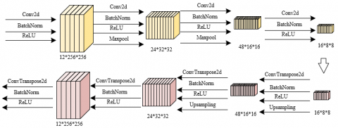
For the prediction of thermal distortion in the LPBF process, a model consisting of two feature extraction networks, a LPBF condition feature extraction network, a product shape feature extraction network, and a Decoder network was designed.
Figure 3. Structure and hyperparameters of the dual-field feature extraction network
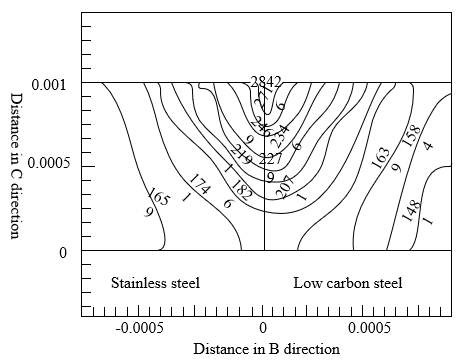
Figure 4. The product shape feature extraction network fitting shape curves
Figure 3 illustrates the structure and hyperparameters of the dual-field feature extraction network. The networks adopts a multi-layer convolutional neural network (CNN) structure, with each layer consisting of convolutional layer, pooling layer, and activation function, aiming to extract key features from the thermal flow field and stress field. Raw data from the thermal flow and stress fields serve as the input, and the output is the high-level feature vectors of the thermal flow and stress fields. The feature extraction network for LPBF conditions is a deep neural network (DNN) made up of densely connected layers, extracting and learning key features of LPBF conditions. The input to this network is the parameters of LPBF, and the output is the high-level feature vectors of these conditions. A CNN is employed for the product shape feature extraction network, targeting the extraction of key features of the product shape. The input here is the shape description of the product, while the output is its high-level feature vector. Figure 4 provides a schematic of the product shape feature extraction network fitting the shape curves.
The Decoder network comprises multiple fully connected DNN layers, including a Dropout layer to prevent overfitting and a Batch Normalization layer for normalization. High-level feature vectors from the three network modules serve as the input, with the predicted product thermal distortion values or metrics being the output.
A profound exploration was conducted into the construction of the dual-field models during the LPBF process, and an in-depth study was undertaken regarding the analysis of flow and heat transfer in the melt pool using both laminar and turbulent models. Based on the figure above, the following analysis can be made. Figure 5 (1) (Turbulent Model) displays a more complex flow structure, which is consistent with the inherent characteristics of turbulence. In turbulent flow, irregular motion is observed, with numerous vortices and mixings present, leading to a more uniform temperature distribution within the melt pool. On the other hand, Figure 5 (2) (Laminar Model) showcases a more regular and smooth flow pattern, with isotherms appearing more concentrated and continuous. This suggests that, under laminar conditions, the heat in the melt pool primarily propagates along certain specific paths. In the turbulent model, a more uniform distribution of isotherms is observed, implying that the heat distribution in the melt pool is relatively even, aiding in reducing local overheating or cooling phenomena. In contrast, under the laminar model, the distribution of isotherms is more concentrated, indicating a noticeable temperature gradient within the melt pool, which can result in insufficient or excessive melting in specific regions of the workpiece.
(1) Turbulent flow
(2) Laminar flow
Figure 5. Isotherms of the melt pool cross-section
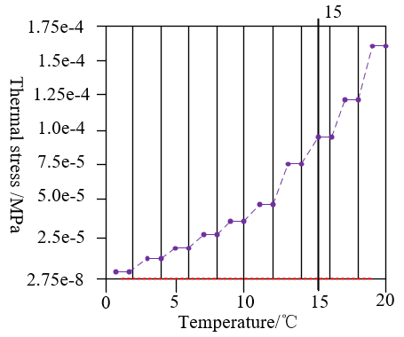
Figure 6. Relationship curve between thermal stress and temperature
Based on Figure 6, the following analysis can be drawn. In the graph, the red line represents the variation in temperature, while the purple line denotes the change in thermal stress. Initially, an increase in temperature is accompanied by a rise in thermal stress, displaying a directly proportional relationship. However, beyond a certain point in time, even as the temperature continues to ascend, a decline in thermal stress is observed, indicating an inversely proportional relationship with temperature. This trend can be attributed to internal structural changes in the material upon reaching a specific threshold temperature, leading to a reduction in thermal stress. From prior discussions, it is known that during the LPBF process, the formation and cooling rate of the melt pool have implications on the material's internal structure and stress. In the figure, even as the temperature keeps increasing upon reaching a peak, a drop in thermal stress is detected. This phenomenon suggests that at this particular temperature, the material undergoes a phase transition or some form of structural rearrangement, resulting in a decrease in thermal stress. Once the temperature peaks and begins its descent, a rapid drop in thermal stress is also observed, signifying stress relief within the material during the cooling process. Thus, it can be concluded that the relationship between temperature and thermal stress in the LPBF process is not simply linear. While they share a direct correlation in the initial stages, an inverse relationship emerges after a certain threshold temperature is attained. Such patterns are closely related to changes in the material's internal structure, phase transitions, or other thermodynamic processes. To ensure the quality and performance of the product, meticulous control over heating and cooling rates, as well as the corresponding temperature and stress distribution, during the LPBF process is deemed imperative.
From Table 1, distinct differences in thermal stress, temperature, and overall deformation between low carbon steel and stainless steel can be observed under identical laser power and cooling water flow rates. A notably higher maximum equivalent stress and thermal stress in low carbon steel compared to stainless steel is noted, attributed to the intrinsic properties of the differing materials. Despite a slight difference in peak temperatures between low carbon steel and stainless steel, significant differences in thermal stress and total deformation are evident. This suggests that the intrinsic mechanical properties of materials play a vital role in the generation of thermal stress. In stainless steel samples, an increase in laser power from 400 to 500 led to rises in the maximum equivalent stress, peak temperature, total deformation, and thermal stress. This trend indicates that an increase in laser power augments the heating rate, subsequently affecting temperature, thereby influencing thermal stress and overall deformation. Moreover, when the cooling water flow rate was reduced from 2 to 1 (at consistent laser power) in stainless steel samples, both the peak temperature and thermal stress saw an increase. It can be deduced that a reduction in cooling speed results in elevated temperature and accumulated stress. Therefore, the type of material is determined to significantly influence thermal stress, overall deformation, and peak temperature. Different materials, under identical processing conditions, produce varying levels of stress and deformation. Increases in laser power lead to higher temperatures and thermal stress. Conversely, reductions in cooling speed also result in elevated temperatures and thermal stresses.
From Figure 7, an analysis of these two equivalent thermal strain curves can be conducted. During the manufacturing process Figure 7 (1), a significant increase in equivalent thermal strain is observed as the temperature rises, particularly around 15℃ where a sharp ascent in equivalent thermal strain starts. Upon manufacturing completion Figure 7 (2), a decline in equivalent thermal strain is noted with decreasing temperature, with the declining trend becoming more pronounced below 30℃. At identical temperatures, the equivalent thermal strain values after manufacturing are significantly lower than those during the manufacturing process. This indicates that temperature fluctuations and other associated factors during manufacturing result in higher strain accumulation, but part of this strain is released upon cooling after completion. High-value zones of equivalent thermal strain are primarily found above 15℃ during manufacturing, while upon manufacturing completion, these high-value zones shift to between 25℃ and 30℃. This shift is attributed to the redistribution or elimination of strain during the cooling process. Thus, it can be concluded that equivalent thermal strain curves during and after manufacturing display different trends, especially under the influence of temperature. This highlights the significance of temperature in governing the generation and distribution of thermal strain during the laser melting manufacturing process. Greater accumulation of equivalent thermal strain in higher temperature zones is correlated with material melting, re-solidification, and other temperature-related processes. However, upon manufacturing completion and subsequent cooling, a certain degree of strain release occurs, leading to a decline in equivalent thermal strain. Proper management and control of equivalent thermal strain become paramount during LPBF, as excessive strain can result in cracks, warping, or other detrimental effects. To optimize the manufacturing process, appropriate cooling strategies and parameter settings should be implemented to minimize strain production and accumulation.
A thermal distortion prediction scheme based on the extraction of these dual-field features has been further proposed. This approach, which uses the combination of thermal flow field and stress field features as synergistic inputs, offers a novel perspective for predicting the extent of product thermal distortion. Table 2 presents thermal strain values (a1, a2, a3) at various measurement points under different sample numbers, along with their corresponding target values (b). a1, a2, and a3 denote thermal strain values at distinct measurement points, while b represents a target response amalgamated from these thermal strain values. From the data, it can be observed that when values of a1, a2, or a3 increase, the target value b often shows a tendency to increase as well. This suggests a positive correlation between the thermal strain values and the target response. However, this relationship isn't always linear, as certain samples demonstrate that even with lower thermal strain values, a higher value of b is achieved. This implies the presence of other influencing factors or interactions between measurement points affecting the final target response. A conclusion can be drawn that data in Table 2 showcases the relationship between thermal strain values at different measurement points and the target response, with a general positive correlation between them. The incorporation of features from both the thermal flow field and the stress field for predicting thermal distortion is believed to enhance the prediction accuracy. Such an approach is beneficial because it can take into account a wider range of factors influencing thermal distortion. To achieve a more precise prediction of thermal distortion, a machine learning model has been trained using this data, and efforts have been made to further optimize and validate the performance of the model.
Table 1. Influence of various parameters on thermal stress
|
Sample Material |
Laser Power |
Cooling Water Flow Rate |
Maximum Equivalent Stress |
Peak Temperature |
Total Deformation,10-2mm |
Thermal Stress,10-4mm/mm |
|
Low Carbon Steel |
500 |
2 |
95.3 |
345.26 |
1.6235 |
6.8952 |
|
Stainless Steel |
500 |
2 |
18.9 |
321.47 |
0.9236 |
2.6548 |
|
Stainless Steel |
400 |
2 |
8.56 |
305.36 |
0.7245 |
1.4652 |
|
Stainless Steel |
500 |
1 |
22.31 |
325.89 |
1.1256 |
3.1258 |
Table 2. Training sample data
|
No. |
Thermal Stress Values of Different Measurement Points |
Target Value |
||
|
a1 |
a2 |
a3 |
b |
|
|
1 |
144.3 |
93.2 |
78.2 |
201.5 |
|
2 |
226.3 |
204.3 |
182.3 |
245.8 |
|
3 |
221.4 |
124.3 |
95.4 |
201.5 |
|
4 |
169.3 |
102.5 |
82.4 |
187.3 |
|
5 |
167.5 |
124.6 |
105.8 |
187.3 |
|
6 |
172.3 |
132.4 |
121.8 |
187.3 |
|
7 |
176.5 |
149.8 |
123.9 |
187.3 |
|
8 |
123.5 |
78.2 |
67.2 |
187.3 |
|
9 |
121.3 |
71.7 |
63.9 |
187.3 |
|
10 |
105.8 |
65.3 |
62.4 |
187.3 |
|
11 |
123 |
127 |
151 |
145 |
|
2 |
185 |
159 |
168 |
205 |
|
13 |
223 |
204 |
223 |
256 |
|
14 |
256 |
231 |
227 |
287 |
|
15 |
312 |
287 |
215 |
346 |
Table 3. Comparison of prediction results from different product thermal distortion prediction models
|
Model |
MSE |
MSE |
Model Runtime T |
|
LSTM |
0.03825 |
0.03524 |
13.28s |
|
GRU |
0.03326 |
0.03286 |
12.36s |
|
Highway |
0.03145 |
0.03017 |
11.23s |
|
Atention-CNN-LSTM |
0.02369 |
0.02218 |
23.58s |
|
Atention-CNN-GRU |
0.01785 |
0.01578 |
20.47s |
|
The proposed model |
0.01452 |
0.01369 |
21.39s |
(2) Upon manufacturing completion
Figure 7. Equivalent thermal strain curves
From the Table 3, it is recognized that the Mean Square Error (MSE) is a commonly utilized metric for evaluating model prediction efficacy. A smaller MSE value indicates superior predictive performance. The model proposed in this research possesses the lowest MSE value, suggesting that it provides the best predictive outcome. Regarding model runtime, the Highway model is identified as having the shortest runtime, although its predictive accuracy is not the best. While the Attention-CNN-LSTM model displays relatively good prediction performance, its runtime is the longest. The runtime of the proposed model is found to be close to that of Attention-CNN-GRU, yet with a superior predictive outcome.
In-depth exploration into the thermal flow field and stress field model construction during the LPBF process has been conducted. Detailed analysis using laminar and turbulence models for flow and heat transfer in the melt pool has been carried out. A thermal distortion prediction scheme based on feature extraction from dual fields has been proposed. This approach, taking the combination of thermal flow field and stress field features as synergistic inputs, offers a novel perspective for predicting the degree of product thermal distortion. Experimental results provide several sets of sample data, including thermal stress, temperature, and equivalent thermal strain, which are correlated with product thermal distortion. These datasets lay the foundation for model training and validation. A comparison of various deep learning models, including LSTM, GRU, Highway, Attention-CNN-LSTM, Attention-CNN-GRU, and the model introduced in this research, has been made. Metrics for this comparison encompass MSE and model runtime. Based on MSE outcomes, the proposed model is determined to exhibit optimal performance in predicting thermal distortion.
A successful cooperative modelling of the thermal flow field and stress field using deep learning techniques has been achieved, and based on this, a new method of thermal distortion prediction has been introduced. Experimental results reveal that the introduced model surpasses other comparative models in predicting thermal distortion. Furthermore, this research provides a fresh perspective-predicting product thermal distortion based on the combined features of thermal flow and stress fields, offering significant reference for subsequent studies. In summary, robust technical support and a new research direction for the domain of thermal distortion prediction have been provided by this research.
[1] Ramlatchan, A., Li, Y. (2022). Image synthesis using conditional GANs for selective laser melting additive manufacturing. In 2022 International Joint Conference on Neural Networks (IJCNN), IEEE, pp. 1-8. https://doi.org/10.1109/IJCNN55064.2022.9892033
[2] Mauduit, A., Gransac, H., Pillot, S. (2021). Influence of the manufacturing parameters in selective laser melting on properties of aluminum alloy AlSi7Mg0.6 (A357). Annales de Chimie - Science des Matériaux, 45(1): 1-10. https://doi.org/10.18280/acsm.450101
[3] Staroselsky, A., Acharya, R., Cassenti, B. (2020). Development of unified framework for microstructure, residual stress, and crack propensity prediction using phase-field simulations. International Journal of Computational Methods and Experimental Measurements, 8(2): 111-122. https://doi.org/10.2495/CMEM-V8-N2-111-122
[4] Rabouhi, H., Khelfaoui, Y., Khireddine, A. (2020). Comparative study by image analysis of WC-Co alloys elaborated by liquid phase sintering and hot isostatic pressing. Annales de Chimie - Science des Matériaux, 44(4): 263-269. https://doi.org/10.18280/acsm.440405
[5] Zhou, S.Y., Su, Y., Wang, H., Enz, J., Ebel, T., Yan, M. (2020). Selective laser melting additive manufacturing of 7xxx series Al-Zn-Mg-Cu alloy: Cracking elimination by co-incorporation of Si and TiB2. Additive Manufacturing, 36: 101458. https://doi.org/10.1016/j.addma.2020.101458
[6] Kladovasilakis, N., Charalampous, P., Tsongas, K., Kostavelis, I., Tzovaras, D., Tzetzis, D. (2022). Influence of selective laser melting additive manufacturing parameters in inconel 718 superalloy. Materials, 15(4): 1362. https://doi.org/10.3390/ma15041362
[7] Giganto, S., Martínez-Pellitero, S., Cuesta, E., Zapico, P., Barreiro, J. (2022). Proposal of design rules for improving the accuracy of selective laser melting (SLM) manufacturing using benchmarks parts. Rapid Prototyping Journal, 28(6): 1129-1143. https://doi.org/10.1108/RPJ-06-2021-0130
[8] Xu, Y., Qiu, L., Yuan, S., Wang, Y. (2022). Research on shape memory alloy honeycomb structures fabricated by selective laser melting additive manufacturing. Optics & Laser Technology, 152: 108160. https://doi.org/10.1016/j.optlastec.2022.108160
[9] Bresson, Y., Tongne, A., Selva, P., Arnaud, L. (2022). Numerical modelling of parts distortion and beam supports breakage during selective laser melting (SLM) additive manufacturing. The International Journal of Advanced Manufacturing Technology, 119(9-10): 5727-5742. https://doi.org/10.1007/s00170-021-08501-5
[10] Wegener, K., Spierings, A.B., Teti, R., Caggiano, A., Knüttel, D., Staub, A. (2021). A conceptual vision for a bio-intelligent manufacturing cell for Selective Laser Melting. CIRP Journal of Manufacturing Science and Technology, 34: 61-83. https://doi.org/10.1016/j.cirpj.2020.11.009
[11] Nguyen, D.S., Park, H.S., Lee, C.M. (2020). Optimization of selective laser melting process parameters for Ti-6Al-4V alloy manufacturing using deep learning. Journal of Manufacturing Processes, 55: 230-235. https://doi.org/10.1016/j.jmapro.2020.04.014
[12] Luo, S., Ma, X., Xu, J., Li, M., Cao, L. (2021). Deep learning based monitoring of spatter behavior by the acoustic signal in selective laser melting. Sensors, 21(21): 7179. https://doi.org/10.3390/s21217179
[13] Behnke, M., Guo, S. (2021). Comparison of early stopping neural network and random forest for in-situ quality prediction in laser based additive manufacturing. Procedia Manufacturing, 53: 656-663. https://doi.org/10.1016/j.promfg.2021.06.065
[14] Fathizadan, S., Ju, F., Lu, Y. (2021). Deep representation learning for process variation management in Laser Powder Bed Fusion. Additive Manufacturing, 42: 101961. https://doi.org/10.1016/j.addma.2021.101961
[15] Li, Y., Zhang, B.C., Qu, X.H. (2022). Research progress on the influence of microstructure characteristics of metal additive manufacturing on its corrosion resistance. Journal of Engineering Science, 44(4): 573-589.
[16] Zhang, D., Feng, Z., Wang, C., Liu, Z., Dong, D., Zhou, Y., Wu, R. (2017). Modeling of temperature field evolution during multilayered direct laser metal deposition. Journal of Thermal Spray Technology, 26: 831-845. https://doi.org/10.1007/s11666-017-0554-5
[17] Ouyoussef, N., Moustabchir, H. (2023). Predicting fracture placement and analyzing fatigue life in exhaust manifold systems using Finite Element Analysis. Journal Européen des Systèmes Automatisés, 56(3): 493-499. https://doi.org/10.18280/jesa.560317
[18] Azzawi, M.M., Hadi, A.S., Abdullah, A.R. (2023). Finite element analysis of crankshaft stress and vibration in internal combustion engines using ANSYS. Mathematical Modelling of Engineering Problems, 10(3): 1011-1016. https://doi.org/10.18280/mmep.100335
[19] Deng, T., Li, B., Xuan, F. (2021). Additive manufactured thermal metamaterial devices for manipulating heat flow: Geometric configuration design and SLM-assisted fabrication. Engineering Research Express, 3(2): 025038. https://doi.org/10.1088/2631-8695/ac050f
[20] Zhang, Y., Jin, Y., Chen, Y., Liu, J. (2021). Design a new type of laser cladding nozzle and thermal fluid solid multi-field simulation analysis. Materials, 14(18): 5196. https://doi.org/10.3390/ma14185196