Ahmed Sabah Thaker* | Fawziea M. Hussien![]() | Johain J. Faraj
| Johain J. Faraj![]()
© 2023 IIETA. This article is published by IIETA and is licensed under the CC BY 4.0 license (http://creativecommons.org/licenses/by/4.0/).
OPEN ACCESS
An innovative indirect solar dryer, designed for banana dehydration, was developed and assessed, utilizing the Ansys software for simulation. The system comprises a vacuum tube water heater and a drying chamber, the latter of which incorporates phase-change materials (PCMs), thus enhancing the drying performance. A fan positioned within the chamber synergizes with the PCMs, effectively abbreviating the drying time. Computational simulations were executed to refine the system design and operational parameters. A sorption isotherm was constructed to delineate the optimal moisture content and water activity, fundamental parameters for efficient drying. The integrated solar collector facilitates the transformation of solar energy into heat, while the drying chamber, accommodating two baskets of produce, optimizes the heat distribution. Our system demonstrated the capacity to generate high drying temperatures, especially efficient for items exhibiting lower moisture content than bananas. The system achieved a predicted maximum efficiency of 67.40%, operating optimally within a temperature range of 60-65℃. Experimental results were congruent with computational simulations, reinforcing the efficacy of the drying chamber. This study introduces a novel, sustainable method for efficient fruit dehydration, spotlighting its potential applicability beyond bananas to other produce.
indirect solar dryer, moisture content, drying rate, PCM, ANSYS, numerical
The physical principles underlying the processes in conventional and solar dryers are fundamentally similar, employing either high or low temperature techniques. High temperature dryers necessitate precise controls to prevent the adverse effects of over-drying [1]. An early application of elevated temperatures during dehydration can induce surface hardening or cooking in certain foods, while the interior retains residual moisture. Conversely, low-temperature methods find their primary applications in bulk food storage, particularly with cereals, and in scenarios where preservation of color and specific nutrients is paramount [2]. Both active and passive dryers necessitate a multicomponent drying structure. Active solar dryers, which employ blowers for comprehensive convection, are predominantly found in developed regions. Passive dryers, in contrast, leverage wind pressure and solar-heated air for natural convection, offering cost-effectiveness and durability. Chimneys often augment the efficacy of natural convection in these systems [3]. Indirect solar dryers employ thermal energy within a solar collector to circulate heated air around produce. These systems offer various advantages such as increased crop capacity, reduced radiation damage, and a range of drying options. However, their complex designs may necessitate a higher initial investment and skilled labor for loading and product movement [4]. Direct solar dryers, such as cabinet and tent dryers, utilize natural convection within a combined chamber. Constructed from insulated timber boxes, these systems store materials within perforated containers. Portable cabinets are typically composed of wood or metal, while permanent structures may be built using stone, masonry, mud, or concrete [5]. Shortwave solar radiation interacts with crop surfaces, partially reflecting and absorbing, which elevates the temperature, triggers moisture evaporation, and results in moisture loss through long-wavelength radiation and atmospheric conduction [6]. A study investigating a forced convection direct mode solar dryer, equipped with a chimney and a 40W photovoltaic module, dried 50 kg of tomatoes with 90% moisture content in 129 hours, amounting to 55% of the time required for natural sun drying. The outcomes included superior color and flavor, surpassing other solar dryer designs, and extended shelf life [7].
Rabha and Muthukumar [8] evaluated active solar dryers incorporating a paraffin wax-based shell and tube latent heat storage unit. For heating applications, a material was preheated, enabling twenty kilograms of red chill to be dried between 36 and 60 degrees Celsius. During the experiment, air circulated through the tube and shell while the heat storage medium was charged. Heat energy was directed through tubes using a blower and discharged into the drying box. A review by Da Cunha and Eames [9] considered studies examining phase change materials for heat energy storage across various applications. They reported thermal physical properties exceeding 100 degrees Celsius for organic compounds and salt hydrate materials. Subsequent investigations of eutectic mixtures with urea revealed a temperature around 100 degrees Celsius. Eutectic inorganic salt mixtures possessed melting points between 130 and 1250 degrees Celsius, but a sodium and potassium combination, melting at approximately 170 degrees Celsius, exhibited potential for thermal storage utilization.
Jain and Tewari [10] designed a solar dryer exploiting natural convection and storing heat energy for phase transition. The capability of the heat storage material to store thermal energy during the day and release latent heat in the evening enabled the solar dryer to operate an additional 5-6 hours post sunset. In Jodhpur, India, during the month of June, the drying chamber temperature was observed to exceed the ambient air temperature by 6 degrees Celsius in the middle of the night. The economic performance of the dryer, calculated using ideal raw material cost and product sale price, yielded a return on capital of 0.65% and a simple payback period of 1.57 years. Kant et al.'s [11] overview of thermal storage materials, based on the type of heat storage medium, intrigued numerous researchers. The study aimed to develop advanced phase change materials (PCMs) by optimizing thermophysical parameters like thermal conductivity, latent heat of fusion, and sensible heat capacity. The review determined that the phase transition properties of heat storage materials directly influenced the performance of thermal energy storage systems. Mawire et al. [12] employed sunflower oil as a heat transfer medium and a sensible heat storage substance, capitalizing on its widespread availability. The boiling and flash points of sunflower oil were identified as 230 degrees Celsius. The sunflower oil container demonstrated superior storage efficiency (3.0-7.1%) compared to the PCM container (2.5-3.7%). An erythritol-based phase change material cooking pot surpassed the sunflower oil pot due to smaller temperature drops (0.1-9.7℃) from the maximum cooking temperatures over storage cooking times. Furthermore, the erythritol cooker's heat usage efficiency was higher in both cases (4.8-14.3% versus 3.7%-6%).
Bhardwaj et al. [13] conducted an examination of indirect forced convection solar dryers comprising sensible heat storage materials (SHSM) and phase change materials (PCM). In the solar air collector, iron refuse was amalgamated with gravel and motor oil to serve as the SHSM, with RT-42 paraffin functioning as the PCM. According to the results, the original moisture content of 89 percent was reduced to 9 percent. The drying rates for SHSM and PCM were observed to be 0.051 kg/h and 26.1 and 0.81 percent, respectively. In a study by Poblete and Painemal [14], the drying process was scrutinized, employing a gravel bed and air heated by a solar air heater, both with and without sludge derived from the coagulation or flocculation of landfill leachate. The solar energy input per kilogram of sludge was found to be 107.5 kilojoules/kilogram with thermal storage, compared to 240-kilowatt W hours/kilograms without thermal storage and 580.5-kilowatt W hours/kilograms outside the dryer. The energetic efficacy of the drying process was calculated to be 38.13 percent for processes utilizing thermal energy, and without thermal storage respectively, with an overall efficiency of 16.45 percent. Thermal efficiency was determined to be 37.8 percent and 22.2 percent, respectively. Ismaeel and Yumrutaş [15] analyzed a drying system featuring a solar-assisted heat pump linked to an underground thermal energy reservoir and a heat recovery unit. The sun-drying heat pump system consisted of a heat pump, heat recovery unit, flat plate solar collector, drying area, and subsurface thermal energy storage reservoir. A performance analysis model was applied, utilizing heat transfer from a thermal energy storage reservoir to supply heat for the various components of the drying system. The experiment involved measurement and analysis of energy, the rate of evaporation of a given moisture amount, and the temperature of the water in the thermal energy storage reservoir. MATLAB was employed to obtain the findings of the drying system, yielding results of 5.55, 5.28, and 9.25 kg kW-1 h-1 for the heat pump coefficient, system coefficient, and specific moisture evaporation rate, respectively. The experiment was conducted with a 100 kg/h mass flow rate, a 40% can efficiency, a 100 m2 collector area, and a 300 m3 reservoir volume. Yadav and Chandramohan [16] put forth a unique numerical model to evaluate the influence of fins on the thermal energy storage mechanism within an indirect solar dryer. Through simulation, they compared two models, one equipped with fins and the other without, applying an air velocity of 4 m/s in both instances. Case 1 and Case 2 exhibited average emission temperatures of 5.47 K and 9.0 K, respectively. It was revealed that at an air velocity of 1 m/s, both scenarios performed satisfactorily as compared to higher air velocities (2 to 4 m/s). Both systems could sustain operation via the TES device until 10:00 p.m. The average exit temperature of Case I between 4:00 and 10:00 p.m. was 5.47 K above the inlet temperature, while Case II (9.1 K) performed better at an air velocity of 1 m/s. The air in Case II garnered a maximum heat quantity that was 55.2% greater than in Case I at a velocity of 1 m/s. Relative to Case I, Case II exhibited a 6.44 percent higher melting percentage at 1 m/s and an average PCM temperature that was 3.7 K higher.
Objectives of the study:
The dryer is made up of the drying chamber and a phase-change material container. The drying chamber was made from plywood of 20 mm thickness, as shown in Figure 1.
2.1 Dryer details
It was made up of two trays, each measuring 56×46 cm, on which the produce was to be dried. To make cleaning and loading easier, the trays are made to be removable. Stainless steel with perforations was used to create the trays. Because the fruit had a high initial moisture content, stainless steel was chosen to prevent rusting. On the upper surface of the chamber, a 12-centimeter-diameter circular opening was drilled. Through this orifice, hot air was blown into the chamber containing the PCM drying device. A door will offer a way to load and unload the material to be dried at the front of the drying chamber. Screws were used to attach an axial fan to the chamber's output.
Additionally, a heat exchanger was installed in the plenum area (about 10 cm) from the base of the cabinet and was sized according to the lower volume limit. A thermal energy storage (PCM) container that is situated 35 cm above the heat exchanger. This storage area was created to capture heat during water heating and then dissipate it for food product drying. To improve its heat conductivity, the PCM was placed in a copper matrix container. The consistent application of heat was supposed to forestall the food item from becoming rewetted. To ensure that the high temperatures within the dryer were maintained, the drying cabinet and trays were coated a matte black.
Figure 1. Drying chamber
Figure 2 details the current test rig configuration, which includes the following parts:
Figure 2. Flow chart of numerical solution
2.2 Drying process
The examination of complicated events can be done using numerical simulations rather than an expensive prototype and challenging experimental measurements. Numerous engineering issues are needed for the complete Navier-Stokes simulation of complex fluid flows. The answers of conservation continuity, momentum, and energy equations are used to analyse heat transport and fluid flow within the solar collector and dryer. In what follows, we shall describe some numerical methods.
3.1 Equations describing fluids in motion
Both mass and momentum are conserved in fluid motion, which is described by the continuity and momentum equations. Navier-Stokes equations are another name for momentum equations. The conservation of energy in heat transfer fluxes necessitates an additional set of equations. The continuity equation is obtained by applying the law of conservation of mass to a limited differential volume of fluid. The following three equations are obtained in Cartesian coordinates:
3.1.1 Continuity equation (conservation of mass)
The mass change within a control volume must equal the sum of the mass inflow and outflow through the control volume's surface. This can be mathematically expressed as follows for an incompressible fluid.
$\frac{\partial u}{\partial x}+\frac{\partial v}{\partial y}+\frac{\partial w}{\partial z}=0$ (1)
3.1.2 Momentum equation
When the fluid's differential volume is used with Newton's second rule of motion, the resulting momentum equations can be derived. The rate of change of momentum over a given differential volume of fluid is equal to the sum of all external forces acting on that volume, as stated by Newton's second law. The resulting momentum equations [17] are converted by Fluent from Cartesian to cylindrical coordinates and take the following form.
X-Momentum Equation:
$\rho_{n f}\left(u \frac{\partial u}{\partial x}+v \frac{\partial u}{\partial y}+w \frac{\partial u}{\partial z}\right)=-\frac{\partial p}{\partial x}+\mu_{n f}\left(\frac{\partial^2 u}{\partial x^2}+\frac{\partial^2 u}{\partial y^2}+\frac{\partial^2 u}{\partial z^2}\right)$ (2)
Y-Momentum Equation:
$\rho_{n f}\left(u \frac{\partial v}{\partial x}+v \frac{\partial v}{\partial y}+w \frac{\partial v}{\partial z}\right)=-\frac{\partial p}{\partial y}+\mu_{n f}\left(\frac{\partial^2 v}{\partial x^2}+\frac{\partial^2 v}{\partial y^2}+\frac{\partial^2 v}{\partial z^2}\right)$ (3)
Z-Momentum Equation:
$\rho_{n f}\left(u \frac{\partial w}{\partial x}+v \frac{\partial w}{\partial y}+w \frac{\partial w}{\partial z}\right)=-\frac{\partial p}{\partial z}+\mu_{n f}\left(\frac{\partial^2 w}{\partial x^2}+\frac{\partial^2 w}{\partial y^2}+\frac{\partial^2 w}{\partial z^2}\right)$ (4)
3.1.3 Energy equation
According to the first rule of thermodynamics, which is the origin of the energy equation, the rate at which the energy of a fluid particle changes is equal to the rate at which heat is added to the particle plus the rate at which work is done on the particle. The following equation is obtained if it is assumed that the water flow is incompressible and the thermal conductivity value is constant.
$\left(\rho C_p\right)_{n f}\left(u \frac{\partial T_{n f}}{\partial x}+v \frac{\partial T_{n f}}{\partial y}+w \frac{\partial T_{n f}}{\partial z}\right)=K_{n f}\left(\frac{\partial^2 T_{n f}}{\partial x^2}+\frac{\partial^2 T_{n f}}{\partial y^2}+\frac{\partial^2 T_{n f}}{\partial z^2}\right)$ (5)
3.2 Radiation model
An approach to calculating the radioactive transfer equation for a set of discrete angles, where each angle represents a vector with a different address in a global Cartesian system, is provided by the radiation model of discrete ordinates (DO). This model provides for the resolution of radiation conditions in partially transparent walls and spans the complete range of optical thickness. The radioactive transfer equation (RTE) in the direction of s is described by the DO model with a field. The RTE for intensity spectrum I(r,s) as a field equation is:
$\nabla .\left(I_\lambda(\vec{r}, \vec{s}) \vec{s}+\left(a_\lambda+\sigma_s\right) I_\lambda(\vec{r}, \vec{s})\right)=a_\lambda n^2 \frac{\delta T^4}{\pi}+\frac{\delta_s}{4 \pi} \int_0^{4 \pi} I_\lambda(\vec{r}, \vec{s}) \varphi\left(\vec{s}, \vec{s}^{\prime}\right) d \Omega^{\prime}$ (6)
A solar load model is employed in this study to determine the radiation impacts of solar rays that enter a computational area. According to Stephenson [18], if the sky is clear, we may use the following formula to determine the amount of direct normal irradiation (DNI) reaching the Earth's surface:
$\mathrm{I}_{\mathrm{DN}}=\mathrm{A} \,\mathrm{e}^{-\mathrm{B} / \sin \beta}$ (7)
where, A, the perceived extraterrestrial irradiation at m = 0, and B, the atmospheric extinction coefficient, are functions of the date and take into account seasonal changes in the distance between the earth and the sun and the amount of water vapor in the air, respectively. CFD uses these conservation principles over a discretized flow domain to figure out the changes in mass, momentum, and energy that happen when fluid flows from one discrete region to the next.
3.3 Governing equation for PCM domain
FLUENT simulation can be used to address solidification or melting issues in a certain temperature range. Enthalpy-porosity formulation and explicit liquid-solid front tracking are options in FLUENT. The liquid-solid mushy zone or porous zone was disregarded in this closed energy storage device since the fluid component of PCM was fixed within it. This means that the simulation does not use a second equation to account for momentum. The analysis is performed by discretizing the flow domain into cells and then utilizing the finite volume approach. The utilization of discrete cells determines the strategy for solving the governing equations. In order to convert the partial differential equations into algebraic equations, the finite volume approach was employed. Eqs. (8)-(13) express the set of algebraic and differential equations:
Continuity Equation:
$\frac{\partial \rho}{\partial t}+\frac{\partial}{\partial_{x j}}\left[\rho u_j\right]=0$ (8)
Momentum Equation:
$\frac{\partial \rho}{\partial t}\left(\rho u_i\right)+\frac{\partial}{\partial_{x j}}\left[\rho u_i u_j+p \delta_{i j}-\tau_{j i}\right]=0$ (9)
Energy Equation
$\frac{\partial \rho}{\partial t}\left(\rho e_0\right)+\frac{\partial}{\partial_{x j}}\left[\rho u_j e_0+u_j p+q_j-u_i \tau_{i j}\right]=0$ (10)
It was assumed that Stokes' law applied to Newtonian fluids composed of monatomic gases. This leads to the following expression for the viscous stress:
$\tau_{i j}=2 \mu S_{i j}$ (11)
The trace-less viscous strain-rate:
$q_j=-\lambda \frac{\partial T}{\partial x_j}=-C p-\frac{\mu}{p r} \frac{\partial T}{\partial x_j}$ (12)
Table 1. Thermo-physical properties of PCM in the simulation
|
Property |
Units |
Method |
Paraffin |
|
Density |
kg/m3 |
Piecewise continuous |
ρ=2293.6-0.7497 T |
|
Specific heat |
J/kg.K |
Piecewise continuous |
Cp=5806-10.833T+7.2413×10⁻³ T2 |
|
Thermal conductivity |
w/m.℃ |
Constant |
0.25 |
|
Viscosity |
kg/m.s |
Piecewise continuous |
μ=0.4737-2.297×10⁻³+3.731×10⁻⁶T2-2.019×10⁻⁹ T3 |
Fourier’s law heat-flux:
$q_j=-\lambda \frac{\partial T}{\partial x_j}=-C p-\frac{\mu}{p r} \frac{\partial T}{\partial x_j}$ (13)
3.4 Solving processors
Fluent converts the governing equations to algebraic forms that can be solved numerically using a control volume-based technique. This control volume method involves integrating the governing equations within each control volume to generate discrete equations that conserve each quantity on a per-control-volume basis The following values are taken into account for the convergence:
Residual for continuity=10-4
Residual for velocities=10-6
Residual for energy=10-7
For the current circumstances, the SIMPLE algorithm was used to resolve the coupling between the velocity and pressure fields.
3.5 Thermophysical properties of PCM
Table 1 shows materials' thermo-physical characteristics are included in the list of attributes. Thermal energy systems and heat exchanger tubes are made of copper and stainless steel, respectively. The PCM material investigated in this study is paraffin, together with water.
Commercial CFD solution Fluent 18.0 was utilized to run the simulations, with its dedicated solver implementing the finite volume method for the governing equations. The second-order upwind method was used to discretize the convection terms, energy, and the turbulent kinetic and turbulent dissipation energy. This method often guarantees sufficient accuracy, stability, and convergence, especially for trihedral, tetrahedral, and polyhedral mesh flow domains [19]. In ANSYS-Fluent, you can choose from the following five pressure-velocity coupling methods: The non-iterative time advancement (NITA) scheme is used for unstable flows, which necessitates the Fractional Step (FSM) algorithm. The "coupled" system is the only one of these that doesn't derive from the predictor-corrector. The connection between the velocities and pressures was calculated using the SIMPLE method [20].
The Semi-Implicit approach for Pressure-Linked Equations (SIMPLE) is a generally gaussian and accurate approach for calculating pressure. Under the assumption of a uniform pressure distribution, the momentum equation and velocity field are thoroughly discretized over u, v, and w using this method. If the velocity distribution satisfies the continuity equation, then the momentum equation along with the necessary pressure field corrections can be used to attain this objective. Otherwise, a new pressure distribution must be implemented. The following diagram illustrates the stages of the SIMPLE algorithm:
For the entire domain, the pressure field P is estimated. For the full computational area, a plausible pressure distribution P is made as an educated guess. The accurate pressure distribution will be established after multiple iterations, but this pressure distribution will serve as a rough guide.
To determine u∗, v∗, and w∗, solve for momentum. The momentum equations are solved using the assumed pressure distribution from step one. Since u, v, and w are determined by solving the momentum equations, these quantities also define the velocity distribution. This velocity distribution will approximate the precise velocity field.
For the entire domain, determine the pressure correlation P′. We'll contrast a temporal variable denoted by P′. This P′ is computed across the full domain by solving a system of linear algebraic equations. By integrating the mass conservation equation for each control volume with the velocity values determined in step 2, the coefficients for the linear system of equations are determined. The fundamental characteristic of this temporal pressure is that, given the correct pressure and velocity field, the P′ distribution is equal to zero across the entire domain, necessitating the need for future pressure correlation.
Pressure field P should be updated. By including the estimated pressure P′ and the pressure correlation P*, the pressure distribution P is updated as follows:
P=P′+P* (14)
As mentioned earlier, P′=0 if and only if the first-step estimated pressure distribution satisfies the mass conservation equation. More correlations are required based on the supposition that P=P*.
Update u, v, and w using the velocity correlation calculation based on their estimated values:
$\mathrm{u}_{\mathrm{i}}=\mathrm{u}_{\mathrm{i}}^*+\frac{\mathrm{area}}{\mathrm{a}_{\mathrm{p}}}\left(\Delta \mathrm{P}^{\prime}\right)$ (15)
where, $a_p$ is the nodal point coefficient and ∆P′ is the pressure (obtained in step no. 3) acting on each velocity component. The correct velocity field (second term on the right) is obtained by adding the initial velocity field (step No. 2) to a coefficient representing the driving potential for fluid motion.
Calculate any additional variables. Any other scalar variable involved in the problem, such as temperature, concentration, etc., could be estimated once the velocity fields were known.
Verify that the mass conservation equation is satisfied by the flow field solution. The convergence and mass conservation of the step pressure distribution and velocity field are tested. Convergence is achieved when there is little variation in the solution variables from one iteration to the next [21], indicating that all properties have been conserved. The steps are continued until convergence if none of them are met, at which point the operation is resumed using the right pressure P from step No. 1 as the new guessed pressure distribution P. It is important to provide the nodal location for each equation's variable when solving the momentum equation.
The inability to relate the energy equation to the equations of momentum and mass was due to our disregard for buoyancy and our assumption of constant fluid properties. By solving the equations of motion and continuity, we obtained the flow field, and the energy equation yielded the temperature distribution. The estimated residual value of variables like energy, mass, turbulent kinetic energy (k), and turbulent dissipation energy (ε) is used as the convergence criterion.
If the sum of the normalized residuals for all conservation equations and variables is less than the desired residual values, then the numerical simulation has converged. SIMPLE algorithms are shown in Figure 2.
4.1 Solution parameters
It should be noted that effective numerical control and modeling approaches are required for the calculation to stabilize and converge quickly. One major advantage of the FVM is that it does not rely on a particular mesh structure. This means that the method can be applied to a wide range of problems and modeling requirements, from simple to complex. The FVM can handle irregular meshes and can be used to solve problems in 3D. Fluent v. 18 and SolidWork v. 19 were uses the simulation transforms the governing equations into algebraic forms that may be solved numerically using a control volume-based method. The governing equations are contained within the control volumes in this method. This results in control-volume discrete equations [22] in which all quantities are held constant. The following are elements of the parameters for the solution.
4.2 Number of iterations
The solver will go through this many iterations at the most before stopping. The residuals were carefully watched throughout the iterative process. All simulations performed in this research were considered to have reached converged solutions when the residuals from the iterative procedure for all governing equations remained constant over time and the computing error could be ignored. The iteration was then manually stopped. Most of the time, the number of iterations falls between (1400 to 1600).
Figure 3. Residual of numerical simulation for present study
4.3 Convergence criteria
The "convergence criteria" determine how accurate an iterative solution is. This criterion may be based on a value for the discretization equation's residual that is deemed acceptable or on the difference between two successful iterations that is deemed acceptable. During the iterative solutions for the current investigation, the scaled residual for the continuity, velocities, and energy equations is tracked. The following values are taken into account for times of various foods, drying temperatures, and velocities:
Residual for continuity=10- 4
Residual for velocities=10- 6
Residual for energy=10-7
In Figure 3 we can see the convergence history of the continuity, momentum, and energy equations.
5.1 Numerical results observations
This study shows the flow, heat transfer, temperature distribution, velocity contours, and relative humidity contours for the current models using the finite volume technique single-phase model numerical results from the commercial CFD tool Ansys-Workbench 18.0. The outcomes replicate the experimental findings in terms of how relative humidity changes with the time of day and temperature distribution.
5.2 Validation of CFD results
All experiment tests are verified to show that the CFD can forecast fluid flow and heat transfer in the drying chamber. so that we may wrap up the most challenging, intricate, and important aspect of this research. The drying room's simulated drying chamber efficiency are contrasted with those discovered via tests in Table 2. From this table, it can be shown that the simulated values and experimental values agree to within +6%. The experimental losses, which are not taken into account theoretically, may be responsible for this difference. The behavior of both findings is the same, however, and the differences are within reasonable bounds.
Table 2. Experimental and simulated drying chamber efficiencies with PCM for V-Shape container
|
Daytime (h) |
EXP. |
NUM. |
e% |
|
9:00 a.m. |
21.2% |
24.3% |
2.0 |
|
10:00 a.m. |
23.4% |
25.2% |
1.8 |
|
11:00 a.m. |
26.1% |
29.9% |
3.8 |
|
12:00 p.m. |
28.7% |
34.8% |
6.1 |
|
1:00 p.m. |
26.5% |
28.4% |
1.9 |
5.3 Temperature contours
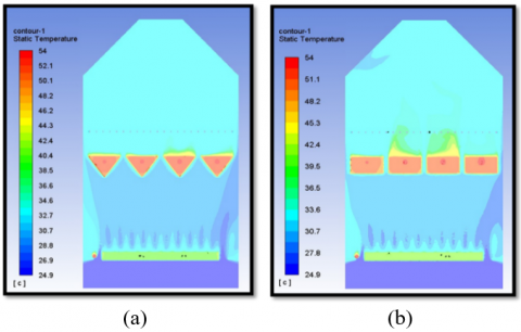
The inclusion of PCM in either a V-shaped or U-shaped container results in a different static temperature distribution along the test section at midplane (dryer chamber), as shown in Figure 4. The maximum temperature degree recorded is 54℃ for a V-shape because the PCM material helps to conserve and accumulate heat, which means decreasing the total drying time. However, because the CFD does not account for wind and other environmental effects during the simulation, there were bound to be some minor discrepancies and variations in temperature. This was not the case with the experimental approach, where the temperatures recorded by sensors can change because of environmental factors. The figure also shows that the U-shape is not efficient enough in heat preservation, which means that the drying time of the fruit will be longer compared to the V-shape. This is because the surface area exposed to heat loss is less than that in the U-shape.
Figure 5 presents static temperature contours without the presence of PCM. These temperature contours show decreasing temperatures at the exit in U-shape as compared to V-shape, and the color maps on the left show a 6℃ maximum difference between the container with and without PCM cases, which means less heat transfer.
Figure 4. Temperature distribution of dryer surface (a) V-Shape; (b) U- shape container with PCM
Figure 5. Temperature distribution of dryer surface a) V-Shape; b) U- shape container without PCM
5.4 Velocity contours
Figure 6 shows a three-dimensional perspective of the drying chamber with velocity contours over a focal distance of the test section for V-shaped and U-shaped containers. The CFD-Post picture shows that the velocity value near the V-shape container is lower than that in the U-shape container because the triangular shape works to hinder the speed of the flowing air, but the speed begins to increase as we approach the exit of the drying chamber due to space narrowing. In fact, the average velocity of the outgoing air does not change with the presence of PCM. The distribution was not even across the two trays, and the top tray dried faster than the bottom tray. This was also observed in studies where banana slices placed on the bottom tray took longer to dry than those placed on the top tray. The hot air exit port should be positioned in the middle of the drying chamber rather than at the top to address this issue and improve performance. This phenomenon has caused banana slices to dry properly and uniformly, shortening the time it takes for banana fruits to dry.
Figures 6. Velocity contours in (m/s) for a) V-Shape; b) U- shape container
Figures 7. Relative humidity contours in (%) for a) V-Shape; b) U- shape container with PCM
Figures 8. Relative humidity contours in (%) for a) V-Shape; b) U- shape container without PCM
5.5 Relative humidity contours
Figure 7 shows volume rendering and humidity distributions across trays within the drying chamber. The relative humidity in the drying chambers was estimated using the fluent approximation discussed in the previous chapter. The following data were obtained with respect to each V-shape and U-shape, respectively. The relative humidity is in %, and the time is in hour format. With the presence of PCM, the relative humidity for U-shape is higher than that for V-shape by 3%, which means a longer drying time for the fruit. Figure 8 demonstrates the relative humidity contours for two physical shapes without PCM. The absence of PCM from the container leads to a significant decrease in relative humidity because this substance is an additional heat source that helps increase the humidity inside the drying room, which means that the time required to dry the fruit will be very long compared to the presence of PCM.
The design and construction of a low-cost forced convection solar drier with evacuated tube solar collector is capable of drying bananas. Experimental and numerical methods were used to evaluate the general performance of the developed solar drier with solar collector and convective air-drying chamber.
6.1 The key findings
1- The maximum efficiency of the solar collector was obtained to be 67.40% which fairly promising that the dryer can generate enough drying temperature for even other products with lower moisture content than banana fruits.
2- The average initial moisture content of a banana ranges from 82-86% (w.b), this value was dropped down to an average of less than 20% final moisture content depending on the solar radiation and loading capacity of the dryer.
3- The optimal drying temperature designed for this dryer is between 60℃ and 65℃. During experiment this temperature reached optimal drying temperature within short time and sometimes went up by 1℃ to 6℃.
6.2 Suggestions for future research
The goal of the current study was to evaluate the thermohydraulic performance of a drying chamber's heat transfer enhancement. This study also paved the way for future studies that aim to gain new knowledge about the processes behind heat transfer enhancement and shorten food drying times. Therefore, it is suggested that the following be included in future work:
1- Care should be made to prevent drying items at high temperatures for a lengthy period of time in a developed dryer. Deterioration of the product may occur as a consequence. An additional mechanism for adjusting temperature may be added to this dyer in this situation to maintain ideal drying conditions.
2- By using an additional solar heating system to create and maintain drying temperature and velocity, a dryer may also be converted into a hybrid drying system.
3- In order to conduct this study, a dryer-specific solar collector that can be tilted at different angles was created. This design feature will make it easier to conduct future research on the performance of solar collectors in Baghdad at various inclination angles that allow for the maximum solar radiation during a particular region or season.
|
$r^{\rightarrow}$ |
position vector |
|
$s^{\rightarrow}$ |
direction vector |
|
$\vec{{s}'}$ |
scattering direction vector |
|
s |
path length |
|
$a \lambda$ |
absorption coefficient |
|
n |
refractive index |
|
$I \lambda$ |
radiation intensity, which depends on position ($r^ \overrightarrow{ }$) and direction ($s^ \overrightarrow{ }$) |
|
T |
local temperature |
|
Greek symbols |
|
|
$\sigma$ |
Stefan-Boltzmann constant |
|
$\sigma s$ |
scattering coefficient |
|
$\phi$ |
phase function |
|
$\Omega^{\prime}$ |
solid angle |
[1] Ekechukwu, O.V. (1999). Review of solar-energy drying systems I: An overview of drying principles and theory. Energy Conversion and Management, 40(6): 593-613. https://doi.org/10.1016/S0196-8904(98)00092-2
[2] Sinha, N.K., Sidhu, J.S., Barta, J., Wu, J.S.B., Pilar Cano, M. (2012). Handbook of Fruits and Fruit Processing, 2 nd ed. A John Wiley & Sons, Ltd., Publication. https://ubblab.weebly.com/uploads/4/7/4/6/47469791/handbook_of_fruits_&_fruit_processing,_2nd_ed.pdf.
[3] Belessiotis, V., Delyannis, E. (2011). Solar drying. Solar Energy, 85(8): 1665-1691. https://doi.org/10.1016/j.solener.2009.10.001
[4] Ekechukwu, O., Norton, B. (1999). Review of solar-energy drying systems II: an overview of solar drying technology. Energy Conversion and Management, 40(6): 615-655. https://doi.org/10.1016/S0196-8904(98)00093-4
[5] Brenndorfer, B., Kennedy, L., Oswin Bateman, C.O., Trim, D.S., Mrema, G.C., Wereko-Brommy, C. (1987). Solar Dryers - Their Role in Post-Harvest Processing (2nd edn.). The Commonwealth Secretariat, London, 298. https://www.gettextbooks.com/isbn/9780850922820.
[6] Chen, C.R., Sharma, A., Vu Lan, N. (2009). Solar-energy drying systems: A review. Renewable and Sustainable Energy Reviews, 13(6-7): 1185-1210. https://doi.org/10.1016/j.rser.2008.08.015
[7] Medugu, D.W. (2010). Performance study of two designs of solar dryers. Journal of Applied Science Research, 2(2): 136-148. https://www.researchgate.net/publication/267404666_Performance_study_of_two_designs_of_solar_dryers.
[8] Rabha, D., Muthukumar, P. (2017). Performance studies on a forced convection solar dryer integrated with a paraffin wax–based latent heat storage system. Solar Energy, 149: 214-226. https://doi.org/10.1016/j.solener.2017.04.012
[9] Da Cunha, J.P., Eames, P. (2016). Thermal energy storage for low and medium temperature applications using phase change materials: A review. Applied Energy, 177: 227-238. https://doi.org/10.1016/j.apenergy.2016.05.097
[10] Jain, D., Tewari, P. (2015). Performance of indirect through pass natural convective solar crop dryer with phase change thermal energy storage. Renewable Energy, 80: 244-250. https://doi.org/10.1016/j.renene.2015.02.012
[11] Kant, K., Shukla, A., Sharma, A. (2017). Advancement in phase change materials for thermal energy storage applications. Solar Energy Materials and Solar Cells, 172: 82-92. https://doi.org/10.1016/j.solmat.2017.07.023
[12] Mawire, A., Lentswe, K., Owusu, P., Shobo, A., Darkwa, J., Calautit, J., Worall, M. (2020). Performance comparison of two solar cooking storage pots combined with wonder bag slow cookers for off-sunshine cooking. Solar Energy, 208: 1166-1180. https://doi.org/10.1016/j.solener.2020.08.053
[13] Bhardwaj, A., Kumar, R., Chauhan, R. (2019). Experimental investigation of the performance of a novel solar dryer for drying medicinal plants in Western Himalayan region. Solar Energy, 177: 395-407. https://doi.org/10.1016/j.solener.2018.11.007
[14] Poblete, R., Painemal, O. (2020). Improvement of the solar drying process of sludge using thermal storage. Journal of Environmental Management, 255: 109883. https://doi.org/10.1016/j.jenvman.2019.109883
[15] Ismaeel, H.H., Yumrutaş, R. (2020). Thermal performance of a solar‐assisted heat pump drying system with thermal energy storage tank and heat recovery unit. International Journal of Energy Research, 44(5): 3426-3445. https://doi.org/10.1002/er.4966
[16] Yadav, S., Chandramohan, V. (2020). Performance comparison of thermal energy storage system for indirect solar dryer with and without finned copper tube. Sustainable Energy Technologies and Assessments, 37: 100609. https://doi.org/10.1016/j.seta.2019.100609
[17] ANSYS FLUENT 12.0 Theory Guide. ANSYS, Inc. (2009). https://www.afs.enea.it/project/neptunius/docs/fluent/html/th/main_pre.htm.
[18] Stephenson, D.G. (1967). Tables of solar altitude and azimuth; Intensity and solar heat gain tables. Division of Building Research, National Research Council of Canada, Ottawa, Technical Paper No. 243. https://doi.org/10.4224/20378809
[19] Kumar, P. (2011). A CFD study of heat transfer enhancement in pipe flow with Al2O3 nanofluid. World Academy of Science, Engineering and Technology, 57: 746-750.
[20] Versteeg, H.K., Malalasekera, W. (1995). An Introduction to Computational Fluid Dynamics-The Finite Volume Method. Longman Group Ltd. https://www.scribd.com/doc/8650266/Versteeg-H-K-Malalasekera-W-Introduction-to-Computational-Fluid-Dynamics-the-Finite-Volume-Meth.
[21] Quatember, B., Muhlthaler, H. (2003). Generation of CFD meshes from biplane angiograms: An example of image-based mesh generation and simulation. Applied Numerical Mathematics, 46(3-4): 379-397. https://doi.org/10.1016/S0168-9274(03)00043-6
[22] FLUENT Incorporated, FLUENT 5 User’s Guide, Fluent Incorporated Lebanon, NH-USA, 1998. https://www.scirp.org/(S(vtj3fa45qm1ean45%20vvffcz55))/reference/referencespapers.aspx?referenceid=782003.