Sheetal Gonsalves*![]() | Swapna Gabbur
| Swapna Gabbur![]()
© 2023 IIETA. This article is published by IIETA and is licensed under the CC BY 4.0 license (http://creativecommons.org/licenses/by/4.0/).
OPEN ACCESS
This work presents an in-depth examination of heat and mass transfer phenomena in a radiative and chemically reactive magneto-micropolar nanofluid flow under the influence of convective boundary conditions. The governing equations of the model, represented in their non-linear form via Falkner and Skan transformations, are scrutinized using the Finite Element Method (FEM). Validation with existing literature corroborates the precision of the proposed model. Analyses of the results elucidate the impacts of various parameters on the temperature, species concentration, micro-rotation, and velocity characteristics of the system. Notably, an enhancement in the thermal conductivity of the magneto-micropolar nanofluid is observed in correlation with an increased nanoparticles volume fraction. A positive relationship is discerned between the temperature and the parameters for radiation and convective boundary conditions. Furthermore, a decrement in the Schmidt number is associated with an accelerated diffusion rate. The findings derived from this study hold substantial implications for practical applications in diverse fields such as heat and cooling systems, enhanced oil recovery, thermal management in electronics, material processing, and nanofluidics. This research thus contributes to the existing body of knowledge by offering an intricate understanding of the behavior and manipulation of magneto-micropolar nanofluid flow.
magneto-micropolar nanofluid, convective boundary condition, heat mass transfer, chemical reaction, radiation, wedge, FEM
Nanofluid flow is widely recognized for its potential in enhancing heat transfer across industrial and engineering applications, with the conductivity of such fluids being augmented by the introduction of nanoparticles into the base fluid [1]. Investigations into mixed convective nanofluid stagnation point flow have been conducted by Ellahi et al. [2], while Ahmed et al. [3] have examined viscous dissipation and radiative heat flux over a moving wedge utilizing volume fraction. The flow of radiative nanofluids over a wedge has also been considered by Amar and Kishan [4]. Recent studies have expanded upon these aspects of nanofluids under various physical circumstances [5-7].
Fluids exhibiting microstructural properties, such as the gyration of microelements and rotary motions, are extensively utilized across numerous material and chemical engineering processes, slurry technologies, and biomechanics. Eringen [8] proposed the micropolar fluid theory to model these effects. This model has gained substantial popularity due to its ability to accurately replicate a variety of substances, from biological fluids like blood and synovial fluids to smart fluids and various colloidal suspensions [9-11].
Despite its usefulness, the nanofluid model's applicability is restricted due to its inability to explain a class of fluids that exhibit distinctive microscopic characteristics driven by the local structure of fluid particles and microrotation. To address such limitations, Bourantas and Loukopoulos [12] investigated micropolar Al2O3-water based nanofluid flow under magnetic field effects using the Moving Least Squares method. Türk and Tezer-Sezgin [13] employed the Finite Element Method (FEM) to examine micropolar nanofluid free convection flow. Further investigations into micropolar nanofluid models, considering factors such as inclined surfaces, have been carried out by Rafique et al. [14], among others [15-17].
Flows involving chemical reactions are prevalent across numerous fields of engineering research, including cooling towers, nuclear reactor cooling, drying, food processing, and geophysics [18, 19]. Investigations into chemical reactions with convective flows of electrically conducting fluid have garnered significant attention due to their varied applications, ranging from hybrid MHD power generators and geophysics to plasma studies, astrophysical flows, magnetic materials processing, chemical engineering, and nuclear fusion. An understanding of both fluid dynamics and the chemistry of the nanoparticles and base fluid is fundamental to nanofluid research. Chemical reactions can influence the stability, dispersion, thermal characteristics, and catalytic behaviour of nanofluids, thereby playing a pivotal role in understanding and optimizing magneto-micropolar nanofluid flow. The boundary layer theory has been employed by numerous authors [20-23] to investigate various aspects of transport phenomena.
Heat and mass transfer often occur simultaneously, involving multiple species diffusion across fluid. Due to its vast range of applications in materials fabrication, mechanical, nuclear, and chemical processes, significant interest has been directed towards mathematical models that simulate the collective impact of chemical reaction and mass transport in electromagnetic fields [24]. Several authors have conducted comprehensive studies of the convective heat and mass exchange in MHD flows [25-27].
This study delves into the examination of heat and mass transport in mixed convective magneto-micropolar nanofluid flow over a wedge, incorporating the influence of convective boundary conditions, thermal radiation, and chemical reaction. A novel model is proposed herein, integrating Eringen's model for microstructural rheological properties, Rosseland's flux model for thermal radiation effects, and the Tiwari-Das model for simulating nano-scale properties. A first-order chemical reaction is introduced into the conservation of species diffusion equation to formulate the non-linear model. The proposed model provides insights into the influence of various factors determining the flow regime, achieved through the application of a novel finite element code. This research contributes to the existing body of engineering science literature on magneto-micropolar nanofluid by introducing a flow model that has not been previously presented in the literature.
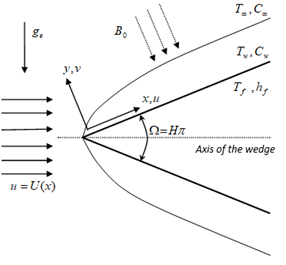
Figure 1 depicts the two-dimensional, steady, laminar, incompressible thermally radiative and chemically reactive magneto-micropolar nanofluid mixed convective flow with the x axis taken along the wedge surface and y axis is normal to it. The wedge surface with temperature Tw (greater than temperature of micropolar nanofluid T∞) is in contact with hot fluid maintained at temperature Th, with coefficient of heat transfer hf which heats the wedge surface.
The velocity components (u, v) are along (x, y). Along y direction variable magnetic field $B(x)=B_0 x^{(m-1) / 2}$ is applied. The species concentration Cw is assumed to be higher than concentration C∞.
Figure 1. Model physical sketch
Following the work El-Dawy and Gorla [28] the mathematical model is:
$u_x+v_y=0$ (1)
$\begin{aligned} & \rho_{n f}\left(u u_x+v u_y\right)=\left(\mu_{n f}+\kappa\right) u_{y y}+\kappa N_y+\sigma_{n f} B^2(U-u) +\left(g_e \beta_{n f}\left(T-T_{\infty}\right)+g_e \beta_{n f}^*\left(C-C_{\infty}\right)\right) \sin \left(\frac{\Omega}{2}\right)+U \frac{d U}{d x}\end{aligned}$ (2)
$u j_x+v j_y=0$ (3)
$\rho_{n f} j\left(u N_x+v N_y\right)=\frac{\partial}{\partial y}\left(\gamma_{n f} N_y\right)-\kappa\left(2 N+u_y\right)$ (4)
$u T_x+v T_y=\alpha_{n f} T_{y y}-\frac{1}{\left(\rho C_p\right)_{n f}} q_y^*$ (5)
$u C_x+v C_y=D_{n f} C_{y y}-\left(C-C_{\infty}\right) k_1$ (6)
velocity field boundary conditions:
$\begin{aligned} & y=0: v=-v_0, u=S, j=0, N=-n u_y, C=C_w \\ & y \rightarrow \infty: u \rightarrow U(x), N \rightarrow 0, C \rightarrow C_{\infty}\end{aligned}$ (7)
boundary conditions for thermal field:
$\begin{aligned} & y \rightarrow 0:-\left(k_{n f}\right) T_y=h_f\left[T_h-T_w\right] \\ & y \rightarrow \infty: T \rightarrow T_{\infty}\end{aligned}$ (8)
Here, wedge angle parameter is $m=\frac{H}{2-H}$, $\frac{H=\Omega}{\pi}$ and $U(x)=$ $b x^m$ is free stream velocity. Unfavourable pressure gradient is denoted by -H whereas if it is positive, it signifies favourable pressure gradient. The pressure distribution outside boundary-layer gets affected by variations in m. Therefore, solutions derived for various values of m are helpful to illustrate how boundary-layer responds to pressure gradient. The flow outside of boundary-layer is boosted by positive wedge angle. For radiation, Rosseland’s approximation is applied where $q^*=-\frac{4 \sigma^*}{3 k^*}\left(\frac{\partial}{\partial y} T^4\right)$ is radiative heat flux. By referring Mohyud-din et al. [29], we have $q^*=-\frac{16 \sigma^* T_{\infty}^3}{3 k^*} T_y$. Also, $\gamma_{n f}(x, y)=\left(\mu_{n f}+\frac{\kappa}{2}\right) j(x, y)$ is spin gradient viscosity and thermophysical characteristics of nanofluid are referred from Devi and Devi [30].
Proceeding with the analysis, define $v=-\Psi_x, u=\Psi_y$ to satisfy Eq. (1), where, $\Psi(x, y)$ defines the stream function.
Introduce the dimensionless quantities as:
$\begin{aligned} & \eta=\left(\frac{U(1+m)}{2 x v_f}\right)^{\frac{1}{2}} y, \Psi=\left(\frac{2 v_f x U}{(1+m)}\right)^{\frac{1}{2}} f(\eta), \\ & N=\left(\frac{(1+m) U^3}{2 v_f x}\right)^{\frac{1}{2}} g(\eta), j=\left(\frac{2 v_f x}{(1+m) U}\right) i(\eta), \\ & \theta(\eta)=\frac{T-T_{\infty}}{T_h-T_{\infty}}, \varphi(\eta)=\frac{C-C_{\infty}}{C_w-C_{\infty}} .\end{aligned}$ (9)
We have,
$\begin{aligned} & u=U f^{\prime}(\eta) \\ & v=-\left(\frac{v_f U}{2 x(1+m)}\right)^{\frac{1}{2}}\left[\eta(m-1) f^{\prime}(\eta)+(m+1) f(\eta)\right]\end{aligned}$ (10)
Using Eqs. (9) and (10), Eqs. (1)-(6) get transformed to non-linear ODE.
$\begin{aligned} & \left(\phi_7+K\right) f^{\prime \prime \prime}+\phi_2 M\left(1-f^{\prime}\right)+\phi_1 f f^{\prime \prime}-\frac{2 m}{1+m}\left(\left(f^{\prime}\right)^2-1\right) +K g^{\prime}+\left(\phi_3 \lambda \theta+\phi_4 \lambda_c \varphi\right) \frac{2}{1+m} \sin \frac{\Omega}{2}=0,\end{aligned}$ (11)
$f i^{\prime}=\phi_6 f^{\prime} i$ (12)
$\left(\phi_7+\frac{K}{2}\right)\left(g^{\prime} i\right)^{\prime}-\left(2 g+f^{\prime \prime}\right) K+\phi_1 i\left(f g^{\prime}-\phi_8 f^{\prime} g\right)=0$ (13)
$\left(\frac{k_{n f}}{k_f}+\frac{4}{3} R d\right) \theta^{\prime \prime}+\phi_5 \operatorname{Pr} f \theta^{\prime}=0$ (14)
$(1-\phi) \varphi^{\prime \prime}+S c f \varphi^{\prime}-\frac{2}{1+m} S c C h \varphi=0$ (15)
Here,
$\begin{aligned} & \phi_1=\left[1-\phi+\phi\left(\frac{\rho_s}{\rho_f}\right)\right], \phi_2=\left[1+\frac{3(\sigma-1) \phi}{(\sigma+2)-(\sigma-1) \phi}\right], \\ & \phi_3=\left[1-\phi+\phi \frac{(\rho \beta)_s}{(\rho \beta)_f}\right], \phi_4=\left[1-\phi+\phi \frac{\left(\rho \beta^*\right)_s}{\left(\rho \beta^*\right)_f}\right], \\ & \phi_5=\left[1-\phi+\phi \frac{\left(\rho C_p\right)_s}{\left(\rho C_p\right)_f}\right], \phi_6=\frac{2(1-m)}{1+m}, \\ & \phi_7=\frac{1}{(1-\phi)^{2.5}}, \phi_8=\frac{3 m-1}{1+m} .\end{aligned}$ (16)
Eq. (7) and Eq. (8), becomes:
$\begin{aligned} & f^{\prime}(0)=S, f(0)=s_w, \varphi(0)=1, \\ & g(0)=-n f^{\prime \prime}(0), i(0)=0, \\ & \theta^{\prime}(0)=-a \frac{k_f}{k_{n f}}[1-\theta(0)], g(\infty)=0, \\ & \varphi(\infty)=0, f^{\prime}(\infty)=1, \theta(\infty)=0 .\end{aligned}$ (17)
Here, $a=\frac{h_f}{k_f} \sqrt{\frac{2 v_f x}{(1+m) U}}$, $K=\frac{\kappa}{\mu_f}$, $M=\frac{\sigma_f B_0^2 2}{\rho_f b(1+m)}$, $\lambda=\frac{G r_x}{\operatorname{Re}_x^2}$, $G r_x=\frac{g_e \beta_f\left(T_f-T_{\infty}\right) x^3}{v_f^2}$, $\lambda_c=\frac{G r_c}{\operatorname{Re}_x^2}$, $G r_c=\frac{g_e \beta_f^*\left(C_w-C_{\infty}\right) x^3}{v_f^2}$, $S c= \frac{v_f}{D_f}$, $R e_x=\frac{U x}{v_f}$, $\operatorname{Pr}=\frac{\mu_f\left(c_p\right)_f}{k_f}$, $S c=\frac{v_f}{D_f}$, $R d=\frac{4 \sigma^* T_{\infty}^3}{k_f k^*}$ and $C_h=\frac{k_1 x}{U}$. If at body surface, angular velocity and gyration are taken to be equal, Eq. (11) along with Eq. (16), taking A as dimensionless integration constant, microinertia density is obtained as $i=A f^{\phi_6}$.
Taking A=1, Eq. (13) becomes:
$\left(g^{\prime} f^{\phi_6}\right)^{\prime}\left(\phi_7+\frac{K}{2}\right)-K\left(2 g+f^{\prime \prime}\right)+\phi_1\left(f g^{\prime}-\phi_8 f^{\prime} g\right) f^{\phi_6}=0.$ (18)
The skin friction coefficient(cf), Couple stress (cn), Nusselt (Nux) and Sherwood (Shx) number are of practical interest and are defined as:
$\begin{aligned} & c_f=\frac{\tau_w}{\frac{1}{2} \rho_f U^2}, c_n=\frac{\tau_z}{\frac{1}{2} \rho_f U^2}, N u_x=\frac{x q_w}{k_f\left(T_h-T_{\infty}\right)}, S h_x=\frac{x m_w}{D_f\left(C_w-C_{\infty}\right)}\end{aligned},$ (19)
where, mass flux mw heat flux qw, shear stress τw, couple stress τz, are:
$\begin{aligned} & m_w=-D_{n f}\left[C_y\right]_{y=0}, \tau_w=\left[\left(\mu_{n f}+\kappa\right) u_y+\kappa N\right]_{y=0} ,q_w=-\left[k_{n f}+\frac{16 \sigma^* T^3}{3 k^*}\right]\left(T_y\right)_{y=0}, \tau_z=\left[\left(\mu_{n f}+\kappa\right) N_y\right]_{y=0}\end{aligned},$ (20)
Using Eq. (9) in Eq. (20) we get:
$\begin{aligned} & S h_x /\left(\operatorname{Re}_x\right)^{1 / 2}=-\left(\frac{1+m}{2}\right)^{\frac{1}{2}} \varphi^{\prime}(0), \\ & N u_x /\left(\operatorname{Re}_x\right)^{1 / 2}=-\left(\frac{1+m}{2}\right)^{\frac{1}{2}}\left[\frac{k_{n f}}{k_f}+\frac{4}{3} R d\right] \theta^{\prime}(0), \\ & \frac{1}{2} c_f\left(\operatorname{Re}_x\right)^{1 / 2}=\left(\frac{1+m}{2}\right)^{\frac{1}{2}}\left(\frac{1}{(1-\phi)^{2.5}}+\frac{K}{2}\right) f^{\prime \prime}(0), \\ & c_n\left(\operatorname{Re}_x\right)^{1 / 2}=(2(1+m))^{\frac{1}{2}}\left(\frac{1}{(1-\phi)^{2.5}}+K\right) g^{\prime}(0) .\end{aligned}$ (21)
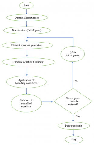
The method utilized here is described in detail by Reddy [31]. The finite-element modeling stages are given in flow chart Figure 2.
Figure 2. FEM flow chart
3.1 Finite element modeling
By employing FEM, nonlinear ODE, Eqs. (11), (14), (15), (18) subject to boundary condition Eq. (17) are evaluated as follows
let:
$f^{\prime}=q$ (22)
The system gets reduced to
$\begin{aligned} & \left(\phi_7+K\right) q^{\prime \prime}+\phi_1 f q^{\prime}+\phi_2 M(1-q) -\frac{2 m}{1+m}\left(q^2-1\right)+K g^{\prime}+\left(\phi_3 \lambda \theta+\phi_4 \lambda_c \varphi\right) \frac{2}{1+m} \sin \frac{\Omega}{2}=0,\end{aligned}$ (23)
$\phi_1\left(f g^{\prime}-\phi_8 q g\right) f^{\phi_6}-K\left(2 g+q^{\prime}\right)+\left(g^{\prime} f^{\phi_6}\right)^{\prime}\left(\phi_7+\frac{K}{2}\right)=0$ (24)
$\left(\frac{k_{n f}}{k_f}+\frac{4}{3} R d\right) \theta^{\prime \prime}+\phi_5 \operatorname{Pr} f \theta^{\prime}=0$ (25)
$(1-\phi) \varphi^{\prime \prime}+S c f \varphi^{\prime}-\frac{2}{1+m} \operatorname{Sc} C h \varphi=0$ (26)
Now, boundary conditions become:
$\begin{aligned} & q(0)=S, f(0)=s_w, \varphi(0)=1, \\ & g(0)=-n q^{\prime}(0), g(\infty)=0, \\ & \theta^{\prime}(0)=-a \frac{k_f}{k_{n f}}[1-\theta(0)], \\ & \varphi(\infty)=0, q(\infty)=1, \theta(\infty)=0 .\end{aligned}$ (27)
3.2 Variational form
Variational form linked with Eqs. (22)-(26), over element $\left(\eta_e, \eta_{e+1}\right)$ is:
$\int_{\eta_{\varepsilon}}^{\eta_{e+1}} w_1\left(f^{\prime}-q\right) d \eta=0$ (28)
$\int_{\eta_e}^{\eta_{e+1}} w_2\left(\begin{array}{l}\left(\phi_7+K\right) q^{\prime \prime}+\phi_1 f q^{\prime}+\phi_2 M(1-q) \\ -\frac{2 m}{1+m}\left(q^2-1\right)+K g^{\prime} \\ +\left(\phi_3 \lambda \theta+\phi_4 \lambda_c \varphi\right) \frac{2}{1+m} \sin \frac{\Omega}{2}\end{array}\right) d \eta=0$ (29)
$\int_{\eta_e}^{\eta_{e+1}} w_3\left(\begin{array}{l}\phi_1\left(f g^{\prime}-\phi_8 q g\right) f^{\phi_6}-K\left(2 g+q^{\prime}\right) \\ +\left(g^{\prime} f^{\phi_6}\right)^{\prime}\left(\phi_7+\frac{K}{2}\right)\end{array}\right) d \eta=0$ (30)
$\int_{\eta_e}^{\eta_{e+1}} w_4\left(\left(\frac{k_{n f}}{k_f}+\frac{4}{3} R d\right) \theta^{\prime \prime}+\phi_5 \operatorname{Pr} f \theta^{\prime}\right) d \eta=0$ (31)
$\int_{\eta_{\varepsilon}}^{\eta_{c+1}} w_5\left((1-\phi) \varphi^{\prime \prime}+\operatorname{Sc} f \varphi^{\prime}-\frac{2}{1+m} \operatorname{Sc} C h \varphi\right) d \eta=0$ (32)
Here, variation in f,q,g,θ and φ are given by weight functions w1, w2, w3, w4 and w5 respectively.
3.3 Finite element form
Taking ψi=w1=w2=w3=w4=w5, with:
$\begin{aligned} f & =\sum_{j=1}^2 f_j \psi_j, q=\sum_{j=1}^2 q_j \psi_j, g=\sum_{j=1}^2 g_j \psi_j, \\ \theta & =\sum_{j=1}^2 \theta_j \psi_j, \varphi=\sum_{j=1}^2 \varphi_j \psi_j,\end{aligned}$ (33)
and linear interpolation functions:
$\begin{aligned} & \psi_1=\left(\eta_{e+1}-\eta_e\right)^{-1}\left(\eta_{e+1}-\eta\right), \\ & \psi_2=\left(\eta_{e+1}-\eta_e\right)^{-1}\left(\eta-\eta_e\right), \quad \eta_e \leq \eta \leq \eta_{e+1}\end{aligned}$ (34)
We substitute Eq. (33) and Eq. (34) into Eqs. (28)-(32), to obtain the finite element model as:
$\left.\begin{array}{llllll}{\left[K^{11}\right]} & {\left[K^{12}\right]} & {\left[K^{13}\right]} & {\left[K^{14}\right]} & {\left[K^{15}\right]} \\ {\left[K^{21}\right]} & {\left[K^{22}\right]} & {\left[K^{23}\right]} & {\left[K^{24}\right]} & {\left[K^{25}\right]} \\ {\left[K^{31}\right]} & {\left[K^{32}\right]} & {\left[K^{33}\right]} & {\left[K^{34}\right]} & {\left[K^{35}\right]} \\ {\left[K^{41}\right]} & {\left[K^{42}\right]} & {\left[K^{43}\right]} & {\left[K^{44}\right]} & {\left[K^{45}\right]} \\ {\left[K^{51}\right]} & {\left[K^{52}\right]} & {\left[K^{53}\right]} & {\left[K^{54}\right]} & {\left[K^{55}\right]}\end{array}\right]\left[\begin{array}{l}\{f\} \\ \{q\} \\ \{g\} \\ \{\theta\} \\ \{\varphi\}\end{array}\right]=\left[\begin{array}{l}\left\{r^1\right\} \\ \left\{r^2\right\} \\ \left\{r^3\right\} \\ \left\{r^4\right\} \\ \left\{r^5\right\}\end{array}\right]$ (35)
Here $\left[K^{m n}\right]_{2 \times 2}$ and $\left\{r^m\right\}_{2 \times 1}$ are matrices given by:
$\begin{gathered}K_{i j}^{11}=\int_{\eta_e}^{\eta_{e+1}} \psi_i \frac{d \psi_j}{d \eta} d \eta, K_{i j}^{12}=-\int_{\eta_e}^{\eta_{e+1}} \psi_i \psi_j d \eta, \\ K_{i j}^{13}=0, K_{i j}^{14}=0, K_{i j}^{15}=0, \\ K_{i j}^{21}=0, K_{i j}^{23}=K \int_{\eta_e}^{\eta_{e+1}} \psi_i \frac{d \psi_j}{d \eta} d \eta, \\ K_{i j}^{24}=\left(\frac{2}{1+m}\right) \phi_3 \lambda \sin \frac{\Omega^{\eta_{e+1}}}{2} \int_{\eta_e}^{\eta_i} \psi_i \psi_j d \eta, \\ K_{i j}^{22}=-\left(\phi_7+K\right) \int_{\eta_e}^{\eta_{e+1}} \frac{d \psi_i}{d \eta} \frac{d \psi_j}{d \eta} d \eta+\phi_1 \int_{\eta_{l_e+1}}^{\eta_{\eta_e}} \bar{f} \psi_i \frac{d \psi_j}{d \eta}d \eta-\phi_2 M \int_{\eta_e}^{\eta_{e+1}} \psi_i \psi_j d \eta \\ K_{i j}^{25}=\left(\frac{2}{1+m}\right) \phi_4 \lambda_c \sin \frac{\Omega^{\eta_{e+1}}}{2} \int_{\eta_e}^{\eta_i} \psi_i \psi_j d \eta, \\ K_{i j}^{31}=0, K_{i j}^{34}=0, K_{i j}^{35}=0, K_{i j}^{32}=-K \int_{\eta_e}^{\eta_{e+1}} \psi_i \frac{d \psi_j}{d \eta} d \eta,\end{gathered}$
$\begin{aligned} & K_y^{33}=-\left(\phi_7+\frac{K}{2}\right) \int_{\eta_e}^{\eta_{e+1}}(\bar{f})^{\phi_6} \frac{d \psi_i}{d \eta} \frac{d \psi_j}{d \eta} d \eta \\ & +\phi_1 \int_{\eta_e}^{\eta_{\eta_i}}(\bar{f})^{\frac{3-m}{1+m}} \psi_i \frac{d \psi_j}{d \eta} d \eta \\ & -\phi_1 \phi_8 \int_{\eta_e}^{\eta_{e+1}}(\bar{f})^{\phi_i} \bar{q} \psi_i \psi_j d \eta-2 K \int_{\eta_e}^{\eta_{e+1}} \psi_i \psi_j d \eta, \\ & K_{i j}^{41}=0, \quad K_{i j}^{42}=0, \quad K_{i j}^{43}=0, \quad K_{i j}^{45}=0, \\ & K_y^{44}=-\left(\frac{k_{\eta f}}{k_f}+\frac{4}{3} R d\right) \int_{\eta_e}^{\eta_{k+1}} \frac{d \psi_i}{d \eta} \frac{d \psi_j}{d \eta} d \eta+\operatorname{Pr} \phi_5 \int_{\eta_e}^{\eta_{k+1}} \bar{f} \psi_i \frac{d \psi_j}{d \eta} d \eta \\ & K_{i j}^{51}=0, \quad K_i^{52}=0, \quad K_i^{53}=0, \quad K_{i j}^{54}=0 \text {, } \\ & K_{i j}^{55}=-(1-\phi) \int_{\eta_e}^{\eta_{e+1}} \frac{d \psi_i}{d \eta} \frac{d \psi_j}{d \eta} d \eta+S c \int_{\eta_e}^{\eta_{e+1}} \bar{f} \psi_i \frac{d \psi_j}{d \eta} d \eta \\ & -\frac{2}{m+1} S c \cdot C h \int_{\eta_e}^{\eta_{e+1}} \psi_i \psi_j d \eta \text {, } \\ & r_i^1=0, \\ & r_i^2=-\left(\frac{2 m}{1+m}+\phi_2 M\right) \int_{\eta_e}^{\eta_{e+1}} \psi_i d \eta-\left(\phi_7+K\right)\left[\psi_i \frac{d q}{d \eta}\right]_{\eta_e}^{\eta_{c+1}} \text {, } \\ & r_i^3=-\left(\phi_7+\frac{K}{2}\right)\left[\psi_i f^{\phi_6} \frac{d g}{d \eta}\right]_{\eta_e}^{\eta_{c+1}}, \\ & r_i^4=-\left(\frac{k_{n f}}{k_f}+\frac{4}{3} R d\right)\left[\psi_i \frac{d \theta}{d \eta}\right]_{\eta_e}^{\eta_{e+1}}, \\ & r_i^5=-(1-\phi)\left[\psi_i \frac{d \varphi}{d \eta}\right]_{\eta_{\tau_c}}^{\eta_{\ell+1}} . \\ & \end{aligned}$
where, $\bar{f}=\sum_{i=1}^2 \bar{f}_i \psi_i, \bar{q}=\sum_{i=1}^2 \overline{q_i} \psi_i$ assumed to be known.
3.4 Convergence criteria
For higher values of η(>8) no substantial alteration in the outcome was seen. Thus, $\infty$ is taken as 8. The domain is divided into n1-linear elements with $h_e=\left(\eta_{e+1}-\eta_e\right)=8 / n_1$. Calculations are run for 50, 100, 150, 200, 240, 320, 400, and 500 elements. The convergence of result is shown in Table 1. It is observed that accuracy is not affected for higher values of n1 (number of elements). Thus, n1=320 is fixed. The order of the element matrix Eq. (35) is 10. If we split domain into 320 equal linear elements, we get matrix of order 1605 after assembling all element equations. The FEM model is non-linear and linearized by using $\bar{f}, \bar{q}$. Subsequently, system of 1599 equations remain after applying the assumed boundary conditions which are solved for $f, q, g, \theta$ and $\varphi$ using iterative scheme. The iterative process is terminated when $\sum_{i, j} \mid \Delta^{n^*+1}-$ $\Delta^{n^*} \mid \leq 10^{-6}$ is satisfied. Here $n^* \Delta=f, q, g, \theta, \varphi$ and iterative steps are denoted by.
Table 1. Convergence of FEM
|
n1 |
f(0.8) |
q(0.8) |
-g(0.8) |
θ(0.8) |
φ(0.8) |
|
50 |
1.320903 |
0.677933 |
0.236291 |
0.009512 |
0.327298 |
|
100 |
1.320962 |
0.677823 |
0.237638 |
0.009875 |
0.328046 |
|
150 |
1.320966 |
0.677815 |
0.237910 |
0.009942 |
0.328183 |
|
200 |
1.320976 |
0.677815 |
0.238008 |
0.009965 |
0.328231 |
|
240 |
1.320980 |
0.677815 |
0.238086 |
0.009983 |
0.328269 |
|
320 |
1.320981 |
0.677815 |
0.238104 |
0.009983 |
0.328269 |
|
400 |
1.320981 |
0.677815 |
0.238104 |
0.009983 |
0.328269 |
|
500 |
1.320981 |
0.677815 |
0.238104 |
0.009983 |
0.328269 |
To evaluate FEM code accuracy and efficiency, the numerical outcomes for $f^{\prime \prime}(0)$, $(1 / 2) c_f\left(R e_x\right)^{\frac{1}{2}}$, $\frac{N u_x}{\left(R e_x\right)^{\frac{1}{2}}}$, $-g(0)$ and $-\theta^{\prime}(0)$ are depicted in Tables 2-4. For comparison study, for Table 2 the parameters are fixed as $\lambda=$ $\lambda_c=C_h=S_w=S=S_c=R d=0$, $a \rightarrow \infty$, $\phi=0$ (pure fluid), $n=1 / 2$, and $P r=1$. For Table 3 fixed values of parameters are $\lambda=\lambda_c=C_h=S_w=S=M=S_c=R d=$ $m=\phi=0$, $a \rightarrow \infty$, $n=1 / 2$, and $P r=1$. For Table 3 parameters are fixed as $\lambda=\lambda_c=n=C_h=s_w=S=M=$ $K=S_c=R d=m=\phi=0$ and $a \rightarrow \infty$.The present outputs show excellent agreement with previous work, there by signifying validity of FEM code.
Table 2. Result of $f^{\prime \prime}(0)$
|
M |
K |
m |
Ishak et al. [32] |
Present Result |
Percent Error |
|
0 |
0 |
0 |
0.3321 |
0.332098 |
0.0006% |
|
1/3 |
0.7575 |
0.757516 |
0.0021% |
||
|
1 |
1.2326 |
1.232605 |
0.0004% |
||
|
1 |
1 |
0 |
0.9599 |
0.959890 |
0.001% |
Table 3. Result of $-\theta^{\prime}(0)$
|
Pr |
Ullah et al. [33] |
Present Result |
Percent Error |
|
1 |
0.3320 |
0.332087 |
0.0262% |
|
10 |
0.7281 |
0.728315 |
0.0295% |
|
100 |
1.5718 |
1.572304 |
0.032% |
Table 4. Results of angular velocity, Nusselt number and skin friction
|
Ishak et al. [34] |
Present Result |
||||||
|
K |
$-g(0)$ |
$\frac{N u_x}{\left(R e_x\right)^{\frac{1}{2}}}$ |
$\frac{1}{2} c_f\left(R e_x\right)^{\frac{1}{2}}$ |
K |
$-g(0)$ |
$\frac{N u_x}{\left(R e_x\right)^{\frac{1}{2}}}$ |
$\frac{1}{2} c_f\left(R e_x\right)^{\frac{1}{2}}$ |
|
0 |
0.2348 |
0.3321 |
0.3321 |
0 |
0.234841 |
0.332104 |
0.332098 |
|
1 |
0.1986 |
0.3147 |
0.4214 |
1 |
0.198676 |
0.314756 |
0.421411 |
|
2 |
0.1730 |
0.3017 |
0.4893 |
2 |
0.173008 |
0.301718 |
0.489307 |
|
4 |
0.1417 |
0.2836 |
0.6014 |
4 |
0.141669 |
0.283632 |
0.601387 |
|
8 |
- |
- |
- |
8 |
0.110590 |
0.264312 |
0.782113 |
The significance of nano-particle concentration (ϕ), material parameter (K), wedge parameter (m) and convective boundary parameter (a), radiation parameter (Rd), Schmidt number (Sc) and chemical reaction parameter (Ch) are explored one at a time while keeping fixed other parameters such as $\operatorname{Pr}=6.2$, $\phi=0.04$, $K=2$, $M=1$, $a=1$, $\lambda=5$, $\lambda_c=1$, $S c=0.5$, $C_h=1$, $n=1 / 2$, $s_w=1$, $R d=1$ and $m=1 / 7$. Also, skin friction, couple stress, Nusselt and Sherwood numbers are reported in Table 5.
Table 5. Numerical values of $f^{\prime \prime}(0)$, $g^{\prime}(0)$, $-\theta^{\prime}(0)$ and $-\varphi^{\prime}(0)$
|
Parameter |
$f^{\prime \prime}(0)$ |
$g^{\prime}(0)$ |
$-\theta^{\prime}(0)$ |
$-\varphi^{\prime}(0)$ |
|
|
Ch |
0.5 |
1.415402 |
0.811744 |
0.35414 |
1.088255 |
|
1 |
1.398951 |
0.798933 |
0.354104 |
1.314672 |
|
|
5 |
1.348052 |
0.758797 |
0.353998 |
2.424784 |
|
|
a |
0.2 |
1.357324 |
0.763415 |
0.07046 |
1.31379 |
|
1 |
1.398951 |
0.798933 |
0.354104 |
1.314672 |
|
|
5 |
1.517157 |
0.900643 |
1.169893 |
1.317155 |
|
|
K |
1 |
1.692567 |
1.127715 |
0.354548 |
1.321971 |
|
2 |
1.398951 |
0.798933 |
0.354104 |
1.314672 |
|
|
4 |
1.075958 |
0.493374 |
0.353518 |
1.305008 |
|
|
m |
0 |
1.107243 |
0.594119 |
0.353582 |
1.364141 |
|
1/7 |
1.398951 |
0.798933 |
0.354104 |
1.314672 |
|
|
1 |
1.70212 |
0.920691 |
0.354631 |
1.135045 |
|
|
Rd |
1 |
1.398951 |
0.798933 |
0.354104 |
1.314672 |
|
2 |
1.411983 |
0.809421 |
0.231473 |
1.315131 |
|
|
3 |
1.420425 |
0.816024 |
0.172432 |
1.315472 |
|
|
Sc |
0.5 |
1.398951 |
0.798933 |
0.354104 |
1.314672 |
|
1 |
1.358615 |
0.767329 |
0.354019 |
2.039688 |
|
|
2 |
1.32473 |
0.740081 |
0.353952 |
3.28865 |
|
|
ϕ |
0.05 |
1.394986 |
0.794502 |
0.354018 |
1.322719 |
|
0.1 |
1.360888 |
0.759366 |
0.353554 |
1.364954 |
|
|
0.3 |
1.234076 |
0.640723 |
0.282460 |
1.461930 |
|
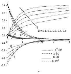
Figure 3. Impact of ϕ on temperature, microrotation, concentration and velocity
Figure 3 displays the temperature, microrotation, concentration and velocity distribution for various ϕ. Throughout the boundary layer, retardation in the velocity and species concentration profiles are marked by increasing nanoparticles volume concentration. This retardation is caused by heavy density of nanoparticles near wedge surface. The temperature rises as concentration increases. This is due to boosting of heat transfer rate by adding high thermal conductivity nanoparticles. Further, it is seen that, at η=1.15 point of inflection is marked closer to the wedge surface. To achieve the appropriate boundary condition, rise in volume concentration causes the microrotation profiles to boost in the first region (η<1.15) and opposite effect can be seen in second region (η>1.15). Therefore, volume fraction is significant in enhancing the thermal conductivity of the liquid.
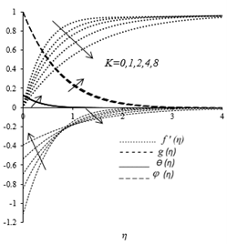
Figure 4 illustrates the temperature, microrotation, concentration and velocity distribution for different K. As K increases, the velocity and microrotation declines while opposite behavior occurs for temperature and concentration. As K increases, fluid motion experiences additional resistive force in linear direction which deteriorate values of $f^{\prime}$. The thermal profiles are enhanced as a result of heating effect that takes place within thermal boundary layer by increasing K.
Figure 5 exhibits the impact of temperature, microrotation, concentration and velocity for different m($0 \leq m \leq 1$). Increasing m boosts the concentration, micro-rotation, velocity and have opposite effect on temperature. Thus, hydrodynamic boundary layer decreases and velocity profile gets closer to wedge surface.
Figure 4. Influence of K on temperature, microrotation, concentration and velocity
Figure 5. Influence of m on temperature, microrotation, concentration and velocity
Figure 6. Influence of a on temperature
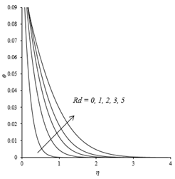
Figure 7. Effect of Rd temperature
Figure 8. Impact of Sc on species concentration
Figure 6 illustrates the impact of a on temperature function. The temperature increases in correlation with a. These results are consistent with the work by Dawar et al. [35]. The magneto-micropolar nanofluid density decreases by a stronger convective heating of the wedge. This produces favorable pressure gradient that simulates the microelements to spin faster and speeds up the flow. It is seen that, at the wedge surface temperature reaches its maxima as hf and thermal resistance are inversely proportional. Further, it is seen from the figure that $\theta(0)=1$ as $a \rightarrow \infty$. The concept of convective boundary parameter is used in physics and engineering to understand and design heat transfer processes in various systems.
Figure 7 depicts the temperature profiles subject to various Rd. For stronger thermal radiation, the temperature of nanofluid rises. The mean absorption coefficient declines if Rd is increased. Due to this radiative heat flux divergence increases, which results in rise in the fluid temperature. Similar trends are observed by Ahmed et al. [3]
Figure 8 depicts impact of Sc on concentration profiles. These profiles become thinner under the influence of Sc. Similar trends are observed by Abdal et al. [36]. The Sc is the ratio of mass to momentum diffusion. Therefore, slower diffusion process is encountered with improvement in Sc which significantly decreases the concentration field and suppress rate of nanoparticles diffusion.
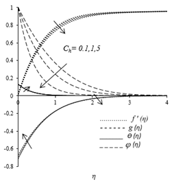
Figure 9 displays the effect of Ch on temperature, microrotation, concentration and velocity profiles. The diffusive transport and flow momentum are delayed by chemical reaction. Hence, as Ch increases velocity decreases. We observe that increasing chemical reaction parameter microrotation increases towards wedge surface whereas it decreases away from surface. A higher chemical reaction parameter causes more effective conversion of chemical energy to thermal energy, this heats fluid and raises the temperature. Concentration profiles declines with surge in chemical reaction parameter. As simulated in Eq. (6), chemical reaction is 1st order destructive and homogeneous. In this reaction nanoparticles undergo a transformation into another species. Consequently, from a physical perspective, it is expected that for more intense chemical reaction the concentration of initial nanoparticles will decrease. The results published by Ramzan et al. [37], Bhatti et al. [38] were found to support these trends. According to Krishnamurthy et al. [39] consumption of chemicals during chemical reactions lowers species concentration.
Figure 9. Influence of Ch on temperature, microrotation, concentration and velocity
Finally, Table 5 presents the impact of ϕ, Ch, a, K, m, Rd, and Sc on Nusselt and Sherwood numbers, skin friction, couple stress. Rising values of a, m, and Rd boost skin friction causing the flow to accelerate, while reverse behavior is observed with the surge in ϕ, Ch, K and Sc. Increment in a, m, and Rd leads to enhance couple stress, whereas it reduces with surge in ϕ, Ch, K and Sc. The Nusselt number is boosted with rise in a, m whereas it reduces with the increase of ϕ, Ch, K, Rd, and Sc. The Sherwood number is elevated with rise in all parameters except wedge angle and material parameter, as K and m have tendency to decrease Sherwood number. Sherwood number is more significantly impacted by the Ch and Sc compared to the other parameters.
This study examines influence of convective boundary on flow of radiative and chemically reacting mixed convection magneto-micropolar nanofluid across permeable wedge. The resulting mathematical model is solved by using FEM. The key observations are:
The flow over a wedge has several potential physical applications in various field of material science, engineering, and energy. The study finds applications in the areas which employ magneto-micropolar nanofluids as their principal heat exchange medium there by making them more efficient for cooling electronics components, industrial machinery, and engines.
|
$a$ |
parameter of convective heat transfer |
|
$C$ |
concentration [kmol m-3] |
|
$C_{\infty}$ |
ambient concentration [kmol m-3] |
|
$C_w$ |
species concentration at surface [kmol m-3] |
|
$C_h$ |
chemical reaction parameter |
|
$D_{n f}$ |
mass diffusivity [m2s-1] |
|
$D_f$ |
mass diffusivity of base fluid [m2s-1] |
|
$f$ |
dimensionless stream function |
|
$g_e$ |
acceleration due to gravity |
|
$g$ |
dimensionless micro-rotation |
|
$G r_x$ |
thermal Grashof number |
|
$G r_c$ |
species Grashof number |
|
$H$ |
Hartre pressure gradient parameter |
|
$i$ |
dimensionless microinertia |
|
$j$ |
microinertia per unit mass |
|
$k_f$ |
thermal conductivity of base fluid |
|
$k_{n f}$ |
thermal conductivity [W/ (K m)] |
|
$k^*$ |
mean absorption coefficient |
|
$K$ |
material parameter |
|
$k_1$ |
rate of chemical reaction [mol m-1s-1] |
|
$M$ |
magnetic parameter |
|
$N$ |
micro-rotation component |
|
$n$ |
micro-gyration parameter |
|
$Pr$ |
Prandtl number |
|
$q$ |
dimensionless velocity |
|
$Rd$ |
radiation parameter |
|
$\operatorname{Re}_x$ |
Reynolds number |
|
$S_w$ |
rate of transpiration at surface |
|
$S c$ |
Schmidt parameter |
|
$T$ |
temperature [K] |
|
$T_h$ |
temperature of hot fluid [K] |
|
$T_{\infty}$ |
ambient temperature [K] |
|
Greek symbols |
|
|
$\sigma$ |
electrical conductivity [s3A2kg-1 m-3] |
|
$\eta$ |
dimensionless coordinate |
|
$\sigma^*$ |
Stephan Boltzman constant |
|
$\beta$ |
thermal expansion coefficient [K-1] |
|
$\beta^*$ |
concentration expansion coefficient [K-1] |
|
$\varphi$ |
dimensionless species concentration |
|
$\theta$ |
dimensionless temperature |
|
$\phi$ |
solid (nanoparticle) volume fraction |
|
$\alpha_{n f}$ |
thermal diffusivity [m2s-1] |
|
$\kappa$ |
micro-rotation viscosity [m2s-1] |
|
$\rho_{n f}$ |
density [kg m-3] |
|
$v_f$ |
viscosity of base fluid [m2s-1] |
|
$\mu_{n f}$ |
viscosity [m2s-1] |
|
$\sigma_{n f}$ |
electrical conductivity of nanofluid |
|
$\rho C_p$ |
heat capacity |
|
$\rho_f$ |
density of base fluid [kg m-3] |
|
$\Omega$ |
total wedge angle |
|
$\lambda$ |
parameter of thermal buoyancy |
|
$\lambda_c$ |
parameter of species buoyancy |
|
Subscripts |
|
|
x |
1st order Partial differentiation with respect to x |
|
y |
1st order partial differentiation with respect to y |
|
yy |
2nd order partial differentiation with respect to y |
|
nf |
nanofluid |
|
f |
Base fluid |
|
Superscript |
|
|
' |
differentiation with respect to $\eta$ |
|
m, n |
matrix dimensions |
|
Acronyms |
|
|
ODE |
ordinary differential equation |
|
FEM |
finite element method |
[1] Choi, S.U., Eastman, J.A. (1995). Enhancing thermal conductivity of fluids with nanoparticles (No. ANL/MSD/CP-84938; CONF-951135-29). Argonne National Lab. (ANL), Argonne, IL (United States).
[2] Ellahi, R., Hassan, M., Zeeshan, A. (2016). Aggregation effects on water base Al2O3-nanofluid over permeable wedge in mixed convection. Asia-Pacific Journal of Chemical Engineering, 11(2): 179-186. https://doi.org/10.1002/apj.1954
[3] Ahmed, N., Tassaddiq, A., Alabdan, R., Adnan, Khan, U., Noor, S., Khan, I. (2019). Applications of nanofluids for the thermal enhancement in radiative and dissipative flow over a wedge. Applied Sciences, 9(10): 1976. https://doi.org/10.3390/app9101976
[4] Amar, N., Kishan, N. (2021). The influence of radiation on MHD boundary layer flow past a nano fluid wedge embedded in porous media. Partial Differential Equations in Applied Mathematics, 4: 100082. https://doi.org/10.1016/j.padiff.2021.100082
[5] N., N., B., V. (2022). MHD nanoliquid flow along a stretched surface with thermal radiation and chemical reaction effects. Mathematical Modelling of Engineering Problems, 9(6): 1704-1710. https://doi.org/10.18280/mmep.090632
[6] Becheri, D., Douha, M. (2023). The buoyancy ratio number effect on Al2O3-water nanofluid magneto convective transport considering Buongiorno model in existence of surface radiation. International Journal of Heat & Technology, 41(1): 72-86. https://doi.org/10.18280/ijht.410108
[7] Gonsalves, S., Swapna, G. (2023). Finite element study of nanofluid through porous nonlinear stretching surface under convective boundary conditions. Materials Today: Proceedings. https://doi.org/10.1016/j.matpr.2023.07.277
[8] Eringen, A.C. (1966). Theory of micropolar fluids. Journal of Mathematics and Mechanics, 16(1): 1-18.
[9] Swapna, G., Kumar, L., Rana, P., Kumari, A., Singh, B. (2018). Finite element study of radiative double-diffusive mixed convection magneto-micropolar flow in a porous medium with chemical reaction and convective condition. Alexandria Engineering Journal, 57(1): 107-120. https://doi.org/10.1016/j.aej.2016.12.001
[10] Islam, A., Das, B., Ali, L.E., Rahman, A. (2022). Numerical study on transient flow of micropolar fluid in a non-darcy porous medium in the presence of magnetic field. International Journal of Heat & Technology, 40(5): 1157-1165. https://doi.org/10.18280/ijht.400506
[11] Usafzai, W.K., Aly, E.H. (2023). Hiemenz flow with heat transfer in a slip condition micropolar fluid model: Exact solutions. International Communications in Heat and Mass Transfer, 144: 106775. https://doi.org/10.1016/j.icheatmasstransfer.2023.106775
[12] Bourantas, G.C., Loukopoulos, V.C. (2014). MHD natural-convection flow in an inclined square enclosure filled with a micropolar-nanofluid. International Journal of Heat and Mass Transfer, 79: 930-944. https://doi.org/10.1016/j.ijheatmasstransfer.2014.08.075
[13] Türk, Ö., Tezer-Sezgin, M. (2017). FEM solution to natural convection flow of a micropolar nanofluid in the presence of a magnetic field. Meccanica, 52: 889-901. https://doi.org/10.1007/s11012-016-0431-1
[14] Rafique, K., Anwar, M.I., Misiran, M., Khan, I., Seikh, A.H., Sherif, E.S.M., Sooppy Nisar, K. (2019). Keller-box simulation for the Buongiorno mathematical model of micropolar nanofluid flow over a nonlinear inclined surface. Processes, 7(12): 926. http://dx.doi.org/10.3390/pr7120926
[15] Rehman, S.U., Mariam, A., Ullah, A., Asjad, M.I., Bajuri, M.Y., Pansera, B.A., Ahmadian, A. (2021). Numerical computation of buoyancy and radiation effects on MHD micropolar nanofluid flow over a stretching/shrinking sheet with heat source. Case Studies in Thermal Engineering, 25: 100867. https://doi.org/10.1016/j.csite.2021.100867
[16] Kausar, M.S., Hussanan, A., Waqas, M., Mamat, M. (2022). Boundary layer flow of micropolar nanofluid towards a permeable stretching sheet in the presence of porous medium with thermal radiation and viscous dissipation. Chinese Journal of Physics, 78: 435-452. https://doi.org/10.1016/j.cjph.2022.06.027
[17] Usafzai, W.K., Aly, E.H., Tharwat, M.M., Mahros, A.M. (2023). Modeling of micropolar nanofluid flow over flat surface with slip velocity and heat transfer: Exact multiple solutions. Alexandria Engineering Journal, 75: 313-323. https://doi.org/10.1016/j.aej.2023.06.004
[18] Levenspiel, O. (1998). Chemical reaction engineering. Industrial & Engineering Chemistry Research, 38(11): 4140-4143. http://dx.doi.org/10.1021/ie990488g
[19] Kamal, F., Zaimi, K., Ishak, A., Pop, I. (2019). Stability analysis of MHD stagnation-point flow towards a permeable stretching/shrinking sheet in a nanofluid with chemical reactions effect. Sains Malaysiana, 48(1): 243-250. http://doi.org/10.17576/jsm-2019-4801-28
[20] Kasmani, R.M., Sivasankaran, S., Bhuvaneswari, M., Siri, Z. (2015). Effect of chemical reaction on convective heat transfer of boundary layer flow in nanofluid over a wedge with heat generation/absorption and suction. Journal of Applied Fluid Mechanics, 9(1): 379-388. http://doi.org/10.18869/acadpub.jafm.68.224.24151
[21] Das, K., Duari, P.R. (2017). Micropolar nanofluid flow over a stretching sheet with chemical reaction. International Journal of Applied and Computational Mathematics, 3: 3229-3239. https://doi.org/10.1007/s40819-016-0294-0
[22] Ali, B., Hussain, S., Nie, Y., Rehman, A. U., Khalid, M. (2020). Buoyancy effetcs on falknerskan flow of a Maxwell nanofluid fluid with activation energy past a wedge: Finite element approach. Chinese Journal of Physics, 68: 368-380. https://doi.org/10.1016/j.cjph.2020.09.026
[23] Pattnaik, P.K., Bhatti, M.M., Mishra, S.R., Abbas, M.A., Bég, O.A. (2022). Mixed convective-radiative dissipative magnetized micropolar nanofluid flow over a stretching surface in porous media with double stratification and chemical reaction effects: ADM-Padé computation. Journal of Mathematics, 2022: 9888379. https://doi.org/10.1155/2022/9888379
[24] Mallikarjuna, B., Rashad, A.M., Chamkha, A.J., Raju, S.H. (2016). Chemical reaction effects on MHD convective heat and mass transfer flow past a rotating vertical cone embedded in a variable porosity regime. Afrika Matematika, 27: 645-665. http://dx.doi.org/10.1007/s13370-015-0372-1
[25] Khan, K.A., Butt, A.R., Raza, N. (2019). Influence of porous medium on magneto hydrodynamics boundary layer flow through elastic sheet with heat and mass transfer. Journal of Nanofluids, 8(4): 725-735. http://dx.doi.org/10.1166/jon.2019.1635
[26] Oyelami, F.H., Falodun, B.O. (2021). Heat and mass transfer of hydrodynamic boundary layer flow along a flat plate with the influence of variable temperature and viscous dissipation. International Journal of Heat and Technology, 39(2): 441-450. https://doi.org/10.18280/ijht.390213
[27] Lawanya, T., Vidhya, M., Govindarajan, A., Priyadarshini, E. (2022). Effect of heat source on MHD flow through permeable structure under chemical reaction and oscillatory suction. International Journal of Heat and Technology, 40(1): 319-325. https://doi.org/10.18280/ijht.400138
[28] El-Dawy, H.A., Gorla, R.S.R. (2021). The flow of a micropolar nanofluid past a stretched and shrinking wedge surface with absorption. Case Studies in Thermal Engineering, 26: 101005. https://doi.org/10.1016/j.csite.2021.101005
[29] Mohyud-din, S.T., Ahmed, N., Khan, U., Rashidi, M.M. (2017). A numerical study of thermo-diffusion, diffusion-thermo and chemical reaction effects on flow of a micropolar fluid in an asymmetric channel with dilating and contracting permeable walls. Engineering Computations, 34(2): 587-602. https://doi.org/10.1108/EC-03-2016-0097
[30] Devi, S.A., Devi, S.S.U. (2016). Numerical investigation of hydromagnetic hybrid Cu–Al2O3/water nanofluid flow over a permeable stretching sheet with suction. International Journal of Nonlinear Sciences and Numerical Simulation, 17(5): 249-257. https://doi.org/10.1515/ijnsns-2016-0037
[31] Reddy, J.N. (2019). Introduction to the Finite Element Method. McGraw-Hill Education.
[32] Ishak, A., Nazar, R., Pop, I. (2006). Boundary-layer flow of a micropolar fluid on a continuous moving or fixed surface. Canadian Journal of Physics, 84(5): 399-410. https://doi.org/10.1139/p06-059
[33] Ullah, I., Khan, I., Shafie, S. (2016). Hydromagnetic Falkner-Skan flow of Casson fluid past a moving wedge with heat transfer. Alexandria Engineering Journal, 55(3): 2139-2148. https://doi.org/10.1016/j.aej.2016.06.023
[34] Ishak, A., Nazar, R., Pop, I. (2009). MHD boundary-layer flow of a micropolar fluid past a wedge with constant wall heat flux. Communications in Nonlinear Science and Numerical Simulation, 14(1): 109-118. https://doi.org/10.1016/j.cnsns.2007.07.011
[35] Dawar, A., Shah, Z., Kumam, P., Alrabaiah, H., Khan, W., Islam, S., Shaheen, N. (2020). Chemically reactive MHD micropolar nanofluid flow with velocity slips and variable heat source/sink. Scientific Reports, 10(1): 20926. https://doi.org/10.1038/s41598-020-77615-9
[36] Abdal, S., Siddique, I., Alshomrani, A.S., Jarad, F., Din, I.S.U., Afzal, S. (2021). Significance of chemical reaction with activation energy for Riga wedge flow of tangent hyperbolic nanofluid in existence of heat source. Case Studies in Thermal Engineering, 28: 101542. https://doi.org/10.1016/j.csite.2021.101542
[37] Ramzan, M., Bilal, M., Chung, J.D. (2017). Radiative Williamson nanofluid flow over a convectively heated Riga plate with chemical reaction-A numerical approach. Chinese Journal of Physics, 55(4): 1663-1673. https://doi.org/10.1016/j.cjph.2017.04.014
[38] Bhatti, M.M., Mishra, S.R., Abbas, T., Rashidi, M.M. (2018). A mathematical model of MHD nanofluid flow having gyrotactic microorganisms with thermal radiation and chemical reaction effects. Neural Computing and Applications, 30: 1237-1249. https://doi.org/10.1007/s00521-016-2768-8
[39] Krishnamurthy, M.R., Prasannakumara, B.C., Gireesha, B.J., Gorla, R.S.R. (2016). Effect of chemical reaction on MHD boundary layer flow and melting heat transfer of Williamson nanofluid in porous medium. Engineering Science and Technology, an International Journal, 19(1): 53-61. https://doi.org/10.1016/j.jestch.2015.06.010