Elson C. Santos*![]() | Emanuel N. Macêdo
| Emanuel N. Macêdo![]() | Rui Nelson O. Magno
| Rui Nelson O. Magno![]() | Marcos A. B. Galhardo
| Marcos A. B. Galhardo![]() | Luís Guilherme M. Oliveira
| Luís Guilherme M. Oliveira![]() | Alaan U. Brito
| Alaan U. Brito![]() | Wilson N. Macêdo
| Wilson N. Macêdo![]()
© 2023 IIETA. This article is published by IIETA and is licensed under the CC BY 4.0 license (http://creativecommons.org/licenses/by/4.0/).
OPEN ACCESS
This study presents a comprehensive exergetic analysis, facilitated by computational modeling, of a solar-powered air conditioning system directly linked to a photovoltaic generator. The system, designed without an energy storage component, aims at addressing the cooling requirements of a library by harnessing the natural regulation of solar energy, under two distinct solar irradiance profiles. Simulations revealed that the photovoltaic generator necessitates a minimum solar incidence of 240 W/m2 to fulfill the basal cooling capacity of the system. The results indicated that only 25% of the library's operational period on a sunny day, and a mere 12.3% on a cloudy day, met the thermal comfort standards for occupants. Furthermore, the study discerned an increase in exergy destruction in the system components over the course of the day. The photovoltaic system exhibited the highest level of exergy destruction, followed by the compressor, condenser, evaporator, and expansion valve respectively. This exergy analysis offers a holistic evaluation of the system's overall efficiency. It transcends mere energy efficiencies and incorporates power quality losses that transpire during the conversion and transport processes. With this in-depth assessment, the study not only identifies the areas of greatest energy losses but also offers insights that could enhance the system's design and operational efficiency.
air conditioning unit, cooling demand, computational modeling, exergetic analysis, photovoltaic system, photovoltaic generator, solar cooling, solar power
The escalating global energy demand necessitates a shift towards renewable energy resources, a paramount determinant of social, economic, and cultural sustainability within urban environments and broader societies [1]. This critical transition to sustainable energy resources is inextricably linked to the concept of sustainable development. This dependency underscores the importance of enhancing energy efficiency in processes that leverage sustainable energy resources [2].
Air conditioning systems, integral for maintaining comfortable and healthy living conditions in regions characterized by severe temperatures or high humidity, contribute significantly to the total energy consumption in buildings [3, 4]. An effective approach to alleviating this energy consumption challenge involves powering these air conditioning systems using photovoltaic solar energy. This strategy transforms solar energy into electricity through photovoltaic solar panels, powering the compressor within the air conditioning system.
Belém, a city situated within the Amazon region, is subject to a typically hot, humid, equatorial climate due to its proximity to the Equator. Consistent high temperatures throughout the year, along with substantial precipitation and humidity, result in minimal variation between daytime and nighttime temperatures. The immense levels of solar radiation incident on buildings, combined with external temperatures exceeding 30℃, often culminate in conditions of thermal discomfort [5].
In contrast to the majority of Brazilian households where electricity is ubiquitously accessible, in many Amazonian localities, electricity - a key facilitator of productive, educational, and leisure activities - is absent, impacting individuals across all age groups [6]. Approximately 425,000 families are bereft of electricity access, rendering the investigation and deployment of photovoltaic solar energy-powered air conditioning systems of considerable interest in various regional locations.
Solar refrigeration, a specific application of renewable energy conversion systems, uses technologies underpinned by photovoltaic solar energy. This application is particularly beneficial as cooling demand tends to align with periods of maximal solar irradiance [7, 8]. The desirability of cooling is significantly magnified in hotter climates compared to cooler regions.
The most prevalent metric for evaluating the efficiency of vapor compression refrigeration systems is the energy efficiency ratio, adjusted to a coefficient of performance [9]. However, exergy analysis, a thermodynamic evaluation technique aimed at assessing energy quality within a system, may be more suitable for ascertaining maximum system performance. This method, used to identify irreversible energy losses in a process, can pinpoint prospective improvement opportunities throughout the system, providing a more realistic perspective of the process [10, 11].
Exergy analysis of an air conditioning system can be conducted by scrutinizing individual system components, identifying the primary exergy destruction points and directing them towards potential improvement areas. Both theoretical and experimental studies have been conducted on air conditioning systems powered by photovoltaic generation.
In terms of coupled systems' behavior, Bilgili [12] theoretically investigated an electric-solar refrigeration system using indirect coupling and battery bank for energy storage. In contrast, Aguilar et al. [13] experimentally examined a photovoltaic energy-powered air conditioning unit, supplemented by conventional energy sources when photovoltaic energy was insufficient.
For numerical analysis and simulation methods, Salilih and Birhane [8] proposed a method for analyzing and simulating a solar-powered vapor compression refrigeration system with a variable-speed compressor directly coupled to the photovoltaic generator. They demonstrated that the hourly variation of exergy mirrors the input power profile of the generator.
Ahamed et al. [14] utilized a thermodynamic analysis better suited for investigating conventionally powered thermal systems' efficiency. They found that exergy depends on evaporation, condensation, subcooling, compressor pressure, and ambient temperature. Anand and Tyagi [15] presented a detailed experimental analysis of the vapor compression refrigeration cycle for different refrigerant charge percentages, while Bayrakçi and Özgür [9] conducted an analysis varying the refrigerant type used.
For combined systems with thermal storage, Mosaffa et al. [16] studied a system comprising latent heat thermal storage and vapor compression refrigeration. They performed an advanced exergy analysis, demonstrating that all unit's exergy destruction is exclusively due to its irreversibilities.
In terms of system performance, Sogut [17] evaluated the exergy and environmental performance of commercially sold air conditioners, while Aman et al. [18] conducted an energy and exergy analysis to evaluate the performance and potential of a solar-powered water and ammonia absorption refrigeration system for residential air conditioning applications.
Although numerous studies have been conducted on solar-powered refrigeration systems, few consider the direct coupling of the air conditioning system with the photovoltaic system. This study addresses this gap, focusing on systems that operate based solely on the availability of the solar resource, without energy storage and auxiliary sources for support.
Moreover, most studies on solar cooling did not employ an exergy analysis to indicate inefficiencies in various components of the air conditioning system and the conversion of solar energy into thermal energy for cooling. The identification of the components contributing most to exergy destruction can guide optimization efforts.
This research represents a significant contribution to the field of air conditioning systems coupled to photovoltaic generators, without energy storage, targeting to meet a small library's cooling demand in the Amazon region. The study employs an exergy analysis approach through computational modeling, examining system performance under different solar irradiance profiles. This analysis provides valuable information to improve efficiency, optimize system design and operation, and guide research and development efforts towards more efficient and sustainable systems.
The photovoltaic air conditioning system (PV-ACS) under study consists of a 1400 Wp photovoltaic generator (PVG), composed of 8 crystalline silicon photovoltaic modules with peak power per module of 175 W (see specifications in Table 1); - a DC-DC converter that increases the DC voltage, suitable for the input voltage level of the ESC, which in turn converts the DC electric current into AC, with an output of 220 V and 60 Hz, suitable for feeding a system of a commercial air conditioner with nominal cooling capacity of 5.28 kW and coefficient of performance (COP) of 3.48. Figure 1 and Table 2 show the configuration of the PV-ACS system and the technical characteristics of the air conditioner. The PVG was considered at an inclination angle of 10 degrees and oriented to the geographic north.
Figure 1. PV-ACS system configuration
Table 1. KC175GT solar panel/module specifications (source- Kyocera)
|
Electrical Performance Under Standard Test Conditions (STC) |
Symbol. |
Rated |
Unity |
|
Maximum power |
Wmax |
175 |
W |
|
Maximum power voltage |
Vm |
23.6 |
V |
|
Maximum power current |
Im |
7.42 |
A |
|
Open circuit voltage |
Voc |
29.2 |
V |
|
Short circuit current |
Isc |
8.09 |
A |
|
Temperature coefficient of Voc |
KV |
-1,09x10⁻¹ |
V/℃ |
|
Temperature coefficient of Isc |
KI |
3,18x10⁻³ |
A/℃ |
|
Module characteristics Length×Width×Depth |
|
(1290×990×36) |
mm |
Table 2. Technical specifications of air conditioning unit - model AR18JSSPSGM/AZ (sourse-Samsung)
|
Technical Specifications |
Symbol |
Rated |
Unity |
|
Cooling Capacity (Min. – Nom. - Max.) |
$\dot{Q}_L$ |
1.61-5.28-6.01 |
kW |
|
Air circulation (cooling) |
VA |
18 |
m3/min |
|
Performance coefficient |
COP |
3.48 |
W/W |
|
Rated power |
$\dot{W}_{e l}$ |
1.5 |
kW |
|
Operating Current |
I |
7.6 |
A |
|
Refrigerant Gas |
|
R410A |
|
|
Type of Compressor |
|
BLDC |
|
|
Test Condition |
Symbol |
Rated |
Unity |
|
Condensing Temp. |
Tcond |
54.4 |
℃ |
|
Evaporating Temp. |
Tev |
7.2 |
℃ |
|
Ambient Temp. |
Ta |
35 |
℃ |
|
Application Envelopes |
Rated |
Tropical |
|
|
Condensing Temp. (℃) |
28 ~ 65 |
28.0 ~ 74.5 |
|
|
Evaporating Temp. (℃) |
-25.0 ~ 12.7 |
||
3.1 Meteorological data
The meteorological data used in this work were obtained in the city of Belém - PA, in the Brazilian Amazon region, whose coordinates are: 1º 27' S, longitude 48º 48' W, and altitude of 16 m, average wind velocity of 1.5 m/s. Data were obtained through a monitoring system (Datalogger) that collects data measured in a meteorological station located in GEDAE, using the following instrumentation: external temperature and relative humidity sensor, model HC2S3, and Kipp & Zonen model CMP6 pyranometer. Irradiance and outside air temperature data for typical sunny and cloudy days are used in this study. Measurements were taken at 10-minute intervals, following the methodology used by Santos et al. [19].
3.2 Modeling the photovoltaic generator
To obtain the I-V characteristic curves of the photovoltaic generator for different irradiance profiles was used the equivalent circuit model shown in Figure 2 [20].
Figure 2. Equivalent circuit of a photovoltaic cell, including the series and parallel resistances
The cell output current is given by Eq. (1). Bana and Saini [21]
$I=I_{P V}-I_0\left[\exp \left(\frac{V+R_S I}{V_t a}\right)-1\right]-\frac{V+R_S I}{R_p}$ (1)
where, Rs and Rp are the equivalent resistances, in series and parallel, respectively, a is the ideality constant of the diode, in the range 1≤a ≤1.5, Carrero et al. [22], being the approximate value of 1.3 for polycrystalline silicon and Vt is the thermal strain of the array, given by Eq. (2).
$V_t=\frac{N_s k T}{q}$ (2)
where, Ns is the number of cells connected in series, k is the Boltzmann constant (1.3806503×10⁻²³ J/K), T is the p-n junction temperature, and q is the electron charge (1.60217646 × 10⁻¹⁹ C).
IPV is the current generated by the light, in amperes, in the standard test condition (Tc,ref= 25℃ e Gref = 1000 W/m²) and is calculated by Eq. (3).
$I_{P V}=\left(I_{P V, n}+K_I \Delta T\right) \frac{G}{G_{r e f}}$ (3)
IPV,n can be calculated as IPV,n=[(Rp+Rs/Rp]Isc,n where Isc,n is the short circuit current, given in Table 1 and $\Delta T=T_c-T_{c, r e f}$, where the solar cell temperature can be obtained from the ambient temperature and is presented in Odeh et al. [23] as shown in Eq. (4)
$T_c=T_a+\frac{G}{800 \mathrm{~W} / \mathrm{m}^2}\left(T_{\text {NOCT }}-20^{\circ} \mathrm{C}\right)$ (4)
Ta is the measured ambient temperature, G is the in-plane irradiance of the generator, and TNOCT is the nominal operating temperature of the solar cell, usually provided by PV module manufacturers.
The saturation current I0 is calculated from Eq. (5). Villalva et al. [20].
$I_0=\frac{I_{s c, n}\,\,+\, K_I \Delta T}{\exp \left(\left(V_{o c, n}\,\,+\,K_V \Delta T\right) / a V_t\right)-1}$ (5)
KI and KV are current and voltage coefficients. Voc,n is the open circuit voltage, found in Table 1.
It is possible to calculate the resistances, Rs and Rp, from an iterative solution proposed by Villalva et al. [20], where the relationship between Rs and Rp, which are the only unknowns in Eq. (1), can be found by making the maximum power calculated by the I–V model of Eq. (1) (Wmax,m) equal to the maximum experimental power, found in the module datasheet (Wmax,e), at the maximum power point MPP, and solving the resulting equation for Rs as shown in Eqs. (6) and (7).
$\begin{gathered}\dot{W}_{\text {máx }, m}=V_m\left\{I_{P V}-I_0\left[\exp \left(\frac{q}{k T} \frac{V_m+R_s I_m}{a N_s}\right)-1\right]-\right. \left.\frac{V_m+R_s I_m}{R_p}\right\}=\dot{W}_{\text {max }, e}\end{gathered}$ (6)
where, Im and Vm are the current and voltage at the maximum power point.
$R_p=\frac{V_m\left(V_m+I_m R_s\right)}{\left\{V_m I_{P V}-V_m I_0 \exp \left[\frac{\left(V_m \, +\, I_m \,\, R_s \,\,\right) q}{N_s a} k T\right]+V_m I_0-W_{\text {max },e \,\,\,}\right\}}$ (7)
According to Pinho and Galdino [24], it is necessary to associate the modules in series or parallel to obtain voltage and current levels suitable for the operation. Similar devices subject to the same irradiance, connected in series, are summed the output voltages while the current remains unchanged, according to Eqs. (8) and (9). In this work, were simulated eight photovoltaic modules connected in series.
$V=\sum_{i=1}^n V_i$ (8)
$I=I_1=I_2=\cdots=I_n$ (9)
3.3 Determination of the maximum power of the generator
A model to determine the maximum power capable of being supplied by a PVG under a given operating condition is suggested by Rawat et al. [25], as shown in Eq. (10).
$\dot{W}_{P V}=P_1 G\left[1+\gamma_m\left(T_c-T_{c, r e f}\right)\right]$ (10)
where, γm corresponds to the temperature coefficient at the point of maximum power; Tc and Tc,ref are the solar cell temperatures under actual and standard test conditions (STC), respectively; G is the irradiance on the generator plane; P1 is the ratio between PVG rated power and the irradiance in the STC, that is, 1,000 W/m2, as shown in Eq. (11).
$P_1=\frac{P_{P V}^0}{G_{r e f}}$ (11)
This model was chosen due to its employability in photovoltaic energy engineering, perfectly meeting the purpose of this work. Furthermore, it considers the two main parameters that affect the PVG output power, the incident irradiance in the generator plane and the temperature of the solar cell.
The power generated by the photovoltaic system ($\dot{W}_{P V}$) is delivered to the set (DC-DC + ESC converter), whose efficiency was equal to 95%. It then activates the ACS compressor electric motor, providing mass flow variation of the refrigerant fluid according to the variation of the power generated.
3.4 Mathematical formulation for exergetic analysis of the photovoltaic system – PV
According to Bayrak et al. [26], the electrical exergy of the photovoltaic system aims to use the present energy as useful energy, where the exergy analysis takes into account the energy quality or capacity and can be expressed by a general balance of photovoltaic exergy, as presented in Eq. (12).
$\sum \dot{E} x_{\text {in }}=\sum \dot{E} x_{\text {out }}+\sum \dot{E} x_{\text {loss }}+\sum \dot{E} x_d$ (12)
where, the input exergy of a photovoltaic system includes only the solar irradiance intensity exergy, as shown in Eqs. (13) and (14) (Bayrak et al. [26] and Petela [27]).
$E x_{i n}=G A\left[1-\frac{4}{3}\left(\frac{T_a}{T_s}\right)+\frac{1}{3}\left(\frac{T_a}{T_s}\right)^4\right]$ (13)
Or
$\dot{E} x_{i n}=\left(1-\frac{T_a}{T_s}\right) G A$ (14)
in which Ts is the temperature of the sun, considered as 5,777 K.
An expression, see Eq. (15), for the output exergy was presented by Bayrak et al. [26] and Joshi et al. [28].
$\dot{E} x_{o u t}=\dot{E} x_{e l}-\dot{E} x_{\text {ther }}$ (15)
Electrical exergy can be expressed according to Eq. (16), presented in Pandey et al. [29].
$\dot{E} x_{e l}=V_{o c} I_{s c}-\dot{E} x_{d, e l}$ (16)
The exergetic loss of electrical energy is presented by Eq. (17).
$\dot{E} x_{d, e l}=V_{o c} I_{s c}-V_m I_m$ (17)
The photovoltaic system thermal exergy, $\dot{E} x_{\text {ther }}$, is constituted by the environment heat loss on the surface of the photovoltaic generator, which can be expressed as shown in Eq. (18) [26, 28, 29].
$\dot{E} x_{t h e r}=\left(1-\frac{T_a}{T_c}\right) \dot{Q}$ (18)
in which $\dot{Q}$ is given by Eq. (19).
$\dot{Q}=h_{c a} A\left(T_c-T_a\right)$ (19)
The heat transfer coefficient hca (convective and radiative) from the solar cell to the environment can be calculated considering the wind velocity (v), the air density, and the surrounding conditions as shown in Eq. (20) [30].
$h_{c a}=5,7+3,8 v$ (20)
Eqs. (15) and (16) include internal and external energy losses, where internal losses are the destruction of electrical exergy, that is, $\dot{E} x_{d, e l}$ and external losses are heat loss, $\dot{E} x_{d, \text { ther }}$ which is numerically equal to $\dot{E} x_{\text {ther }}$ for the PV system [29]. Thus, the loss of exergy in the photovoltaic system is given by Eq. (21), in which the decrease in energy quality is called exergy destroyed or irreversibility.
$\dot{E} x_{d, P V}=\dot{E} x_{d, e l}+\dot{E} x_{t h e r}$ (21)
Using Eqs. (16)-(20) the output exergy of the PV system can be calculated by Eq. (22).
$\dot{E} x_{o u t}=V_m I_m-\left(1-\frac{T_a}{T_c}\right) h_{c a} A\left(T_c-T_a\right)$ (22)
The exergy efficiency of the PV module is described as the ratio of the total output exergy to the total input exergy, presented by Pandey et al. [29], Bayrak et al. [26] and Joshi et al. [28], see Eqs. (23) and (24).
$\eta_{E x, P V}=\frac{\dot{E} x_{o u t}}{\dot{E} x_{i n}}$ (23)
$\eta_{E x, P V}=\frac{V_m I_m-\left(1-\frac{T_a}{T_c}\right) h_{c a} A\left(T_c-T_a\right)}{\left(1-\frac{T_a}{T_s}\right) G A}$ (24)
3.5 Mathematical formulation for exergetic analysis of the vapor compression air conditioning system
Some mathematical formulations are necessary to carry out the analyses, both of energy and exergy for the refrigeration cycle by vapor compression.
The vapor compression system has four main components: evaporator, compressor, condenser, and expansion valve. External energy (power) is supplied to the compressor, and heat is added to the system in the evaporator. In the condenser, heat is rejected from the system.
Exergy losses in various system components are not equal, as shown by Ahamed et al. [14], and Anand and Tyagi [15]. Reference temperature and pressure are denoted by T0 and P0, respectively, and are shown in Table 3.
Table 3. Air conditioning system operating conditions
|
Description |
Symbol |
Value |
Unity |
|
Reference temperature |
T0 |
T0=Ta |
°C |
|
Reference pressure |
P0 |
101.325 |
kPa |
|
Evaporation temperature |
Tev |
10 |
°C |
|
Condensation temperature |
Tcond |
Tcond=Ta+10 |
°C |
|
Isentropic efficiency of the compressor |
ηCI |
Eq. (34) |
% |
|
Mechanical compressor efficiency |
ηCM |
80 |
% |
|
Electric motor efficiency |
ηel |
95 |
% |
Figure 3. Diagram T-s (Temperature-entropy) for the actual steam compression refrigeration cycle
Exergy is consumed or destroyed due to the entropy created as a result of associated processes, according to Sahin et al. [31]. To specify the exergy losses or destructions in the system, in this study, the assumptions considered for the PV-ACS engineering model are:
1. Steady-state conditions are maintained on all components;
2. Pressure losses in the pipes are neglected;
3. Heat gains and losses from or to the system are not considered;
4. Kinetic and potential energy losses are not considered.
In air conditioning systems, heat exchange can be explained based on the T-s diagram shown in Figure 3, where 1-2 is the isentropic compression in the compressor, 2-3, 3-4, and 4-1 are condensation, throttling in the expansion valve and evaporation in the evaporator, respectively.
During a process, the change in the exergy of a system is equal to the difference between the total exergy transfer across the system boundaries and the exergy destroyed within the system boundaries due to irreversibility or entropy production [32]. The overall exergy balance for any type of system and any process is expressed by Eq. (25).
$\dot{E} x_{\text {in }}-\dot{E} x_{\text {out }}-\dot{E} x_d=\Delta E_{\text {system }}$ (25)
where, $\dot{E} x_{\text {in }}$ is the amount of exergy entering a system, $\dot{E} x_{\text {out }}$ is the amount of exergy leaving a system, and $\dot{E} x_d$ is the amount of exergy being destroyed within a system's boundaries. For systems with the steady-state flow, the exergy balance can be expresse Eq. (26).
$\begin{gathered}\dot{E} x_{\text {heat }}-\dot{E} x_{\text {work }}+\dot{E} x_{m a s s, i n}-\dot{E} x_{m a s s, o u t}- \dot{E} x_d=0\end{gathered}$ (26)
Eq. (26) can be expressed in more detail, according to Eq. (27).
$\sum\left(1-\frac{T_0}{T_k}\right) \dot{Q}_k-\dot{W}+\dot{m}\left(\psi_1-\psi_2\right)-\dot{E} x_d=0$ (27)
The mathematical formulation for analysis of exergy in different components is performed according to Ahamed et al. [14], Anand and Tyagi [15], and Bayrakçi and Özgür [9].
The specific exergy, in any state, can be given by Eq. (28).
$\psi=\left(h-h_0\right)-T_0\left(s-s_0\right)$ (28)
The exergy destroyed of the system components is obtained with the exergy balance (availability) described by Eq. (29).
$\dot{E} x_d=\dot{E} x_{i n}-\dot{E} x_{o u t}$ (29)
Considering Eqs. (28) and (29) it is possible to write the first and second laws of thermodynamics for each component of the system.
For the evaporator: The cooling capacity is given by Eq. (30).
$\dot{Q}_L=\dot{m}\left(h_1-h_4\right)$ (30)
in which: h1 (kJ/kg) and h4 (kJ/kg) are the specific enthalpies of states 1 and 4.
The exergy destroyed is given in Eq. (31).
$\dot{E} x_{d, e v}=\dot{m}\left[\left(h_4-h_1\right)-T_0\left(s_4-s_1\right)\right]+\dot{Q}_L\left(1-\frac{T_0}{T_L}\right)$ (31)
where, TL is the temperature of the cold (conditioned) environment.
For the compressor: Compressor power is obtained from Eq. (32).
$\dot{W}_{\text {comp }}=\dot{m}\left(h_2-h_1\right)$ (32)
For a real refrigeration cycle, the specific enthalpy at the compressor output, state two, in Figure 3, is given by Eq. (33).
$h_2=h_1+\frac{h_{2 s-} h_1}{\eta_{C I}}$ (33)
The isentropic compression efficiency ηCI is calculated in Eq. (34) [32].
$\eta_{C I}=0.874-0.0135\left(\frac{P_{c o n d}}{P_{e v}}\right)$ (34)
As presented by Özgoren et al. [33], Pev and Pcond are the evaporating and condensing pressures. For the R410A used in the equipment under study, the Pev assumes the value of 10.85 bar, for Tev equal to 10℃, and the Pcond variable from 20.94 bar to 25.02 bar for Tcond ranging from 35.41℃ to 42.8℃.
The electrical power is given by Eq. (35).
$\dot{W}_{e l}=\frac{\dot{W}_{c o m p}}{\eta_{C M} \,\, \eta_{e l}}$ (35)
The exergy destroyed in the compressor is calculated by Eq. (36).
$\dot{E} x_{d, \text { comp }}=\dot{m}\left[\left(h_1-h_2\right)-T_0\left(s_1-s_2\right)\right]+\dot{W}_{e l}$ (36)
For the condenser: The condensing capacity is given by Eq. (37).
$\dot{Q}_H=\dot{m}\left(h_2-h_3\right)$ (37)
The exergy destroyed in the condenser is given by Eq. (38).
$\dot{E} x_{d, \text { cond }}=\dot{m}\left[\left(h_2-h_3\right)-T_0\left(s_2-s_3\right)\right]-\dot{Q}_H\left(1-\frac{T_0}{T_H}\right)$ (38)
where, TH=Ta
For the expansion valve: The exergy destroyed is given by Eq. (39).
where, h4=h3,
$\dot{E} x_{d, \exp }=\dot{m}\left(s_4-s_3\right)$ (39)
Coefficient of Performance for the refrigeration cycle
The refrigeration cycle performance coefficient (COP) is the relationship between the evaporator cooling capacity and the compressor's electrical energy consumption, given by Eq. (40).
$C O P=\frac{\dot{Q}_L}{\dot{W}_{e l}}$ (40)
And the exergy efficiency is calculated by Eq. (41) [8].
$\eta_{E x, A C S}=\frac{\dot{X}_{Q_L}}{\dot{W}_{e l}}$ (41)
where, $\dot{X}_{Q_L}$ is the rate of positive exergy associated with the removal of heat from the low-temperature medium, which can be obtained by multiplying the Carnot factor ((T0-TL))⁄TL by the cooling capacity $\dot{Q}_L$, where T0, is the reference temperature and TL, is the temperature of the conditioned environment, as presented by Çengel and Boles [34] and used in the work of Salilih and Birhane [8], as presented in Eq. (42).
$\dot{X}_{Q_L}=\frac{T_0-T_L}{T_L} \times \dot{Q}_L$ (42)
3.6 Thermodynamic analysis of the combined system
Figure 4 presents a schematic diagram of the coupling between the PV and ACS systems, called the combined system (sys). According to the Figure 4, the electrical power input to the compressor can be given by Eq. (43).
Figure 4. Schematic diagram of the coupling between the PV and ACS systems
$\dot{W}_{e l}=\dot{W}_{P V} \cdot \eta_{D C-D C} \, \cdot \, \eta_{E S C}$ (43)
Combining Eqs. (10), (32), (33), (35), and (43), we obtain the coupling equation of the combined system Eq. (44) as the variation of the mass flow of the refrigerant from the power generated in the PVG.
$\dot{m}=\frac{P_{F V}^0 \frac{G}{G_{r e f}}\left[1+\gamma_m\left(T_c-T_{c, r e f}\,\, \right)\right] \cdot E f}{\left(h_{2 s}-h_1\right)}$ (44)
where, $E f=\eta_{D C-D C} \cdot \, \eta_{E S C} \cdot \eta_{C M} \cdot \eta_{e l} \cdot \eta_{C I}$.
The COPsys of the combined system (PV-ACS) can be evaluated as in the study of Salilih and Birhane [8] and Kaushik et al. [7], by Eq. (45).
$C O P_{s y s}=\frac{\dot{Q}_L}{G \times A}$ (45)
where, G is the irradiance intensity in (W/m2) and A is the area in (m2) of the photovoltaic module.
The exergy efficiency of the combined system (PV-ACS) can be evaluated by Salilih and Birhane [8] and Kaushik et al. [7], by Eq. (46). For greater precision of the results, it is also possible to evaluate from the input exergy in the PV system (Eq. (14)), as shown in Eq. (47).
$\eta_{E x, s y s}=\frac{E x_{e v}}{E \times A}$ (46)
$\eta_{E x, s y s}=\frac{\dot{X}_{Q_L}}{\left(1-\frac{T_a}{T_S}\right) G A}$ (47)
For the combined system (PV-ACS), the total system exergy destroyed can be estimated according to Eq. (48). The irreversibilities of each refrigeration system component are added to the photovoltaic system irreversibility. Adding the exergy destroyed in each component of the air conditioning system and the photovoltaic generator, an estimate of the total exergy destroyed in the integrated system can be obtained. This measure can be used to assess the efficiency of the system and identify opportunities for improvement in its design and operation.
$\begin{gathered}\dot{E} x_{d, t o t a l}=\dot{E} x_{d, \text { comp }}+\dot{E} x_{d, e v}+\dot{E} x_{d, \text { cond }}+ \dot{E} x_{d, \text { exp }}+\dot{E} x_{d, P V}\end{gathered}$ (48)
3.7 Estimation of the temperature of the environment to be conditioned TL
To simulate the PV-ACS operation, an environment of a small library, with an area of 23 m² and a height of 3 m, located in the GEDAE laboratory, is considered a building with average thermal inertia. The thermal load was calculated for the two analyzed days using the HAP software (Hourly Analysis Program 4.9). The Thermal Loads Table, as well as the library plant, can be found by Santos et al. [19].
To estimate the temperature profile (TL) inside the library from the moment the system starts operating was used the transfer function shown in Eq. (49) [19, 35].
$\sum_{i=0}^1 p_i\left(\dot{Q}_{L, t-\Delta}-T L_{t-i \Delta}\right)=\sum_{i=0}^2 g_i\left(T_r-T_{L, t-i \Delta}\right)$ (49)
where, pi, gi = coefficients of the transfer function, presented in Table 4.
$\dot{Q}_{L, t-\Delta}$= cooling capacity in time t – Δ, (W);
TLt-iΔ= simulated environment’s thermal load in time t – iΔ, (W);
Tr = reference temperature used in calculus of the thermal load, (℃);
TL,t-iΔ = simulated environment’s internal temperature.
Table 4. Normalized coefficients of the transfer function [19]
|
Building Inertia |
$g_0^*$ |
$\boldsymbol{g}_1^*$ |
$\boldsymbol{g}_{\mathbf{2}}^*$ |
$p_0$ |
$p_1$ |
|
W m-2℃-1 |
|||||
|
Light |
9.54 |
-9.82 |
0.28 |
1.0 |
-0.82 |
|
Average |
10.28 |
-10.73 |
0.45 |
1.0 |
-0.87 |
|
Heavy |
10.50 |
-11.07 |
0.57 |
1.0 |
-0.93 |
The normalized coefficients of the transfer function, pi, and gi, can be adjusted to not-null global conductivity coefficients so that they become representatives of the simulated environment, as Eq. (50).
$g_{i, t}=g_i^* \cdot A_{a m b}+p_i\left(U A_{\text {global }}+1.23 \dot{V}_{\text {total }}\right)$ (50)
where, Aamb is the floor’s area, UAglobalis given by Eq. (51), V̇total is the ventilation and infiltration flow to the external environment (l/s) and gi* is presented in Table 4.
$U A_{\text {global }}=U A_{\text {frontages }}+U A_{\text {glasses }}+U A_{\text {roof }}$ (51)
U (W m-2 ℃-1) and A (frontages, glasses, and roof, m²) can be found in Santos et al. [19].
3.8 Estimation of relative humidity inside the conditioned environment (HRL)
To estimate the relative humidity of the air in the conditioned environment, the operation of the ACS is considered as represented in Figure 5.
The process is considered to occur at a steady state, and therefore the mass flow rate of dry air remains constant throughout the process and is given by Eq. (52).
$\dot{m}_{\text {air }}=\frac{A V}{v_{\text {air }}}$ (52)
where, AV is the volumetric flow rate of air circulation, in the amount of 18 m³/min, according to the manufacturer's information, and vair is the specific volume of dry air at inlet 1, which can be obtained by $v_{\text {air }}=\left(\bar{R} / M_{\text {air }}\right)\left(T_1 / P_{\text {air } 1}\right)$, where $\bar{R}=8314 \mathrm{~m}^3 . P a / \mathrm{kmol} . K, M_{\text {air }}=28.97 \mathrm{~kg} / \mathrm{kmol}, T_1$ the inlet temperature of the coil, and $P_{\text {air } 1}$ the partial pressure of dry air, calculated by $P_{\text {air } 1}=P-P_{v 1}$, where $\mathrm{P}$ is the atmospheric air pressure, $P_{v 1}$ is the partial pressure of water atmospheric air pressure, $P_{v 1}$ is the partial pressure of water vapor, given by Eq. (53).
$P_{v 1}=R H_1 \cdot P_{g 1}$ (53)
$R H_1$ is the relative humidity of the air at the inlet of the coil and $P_{g 1}$ is the saturation pressure of the water at temperature $T_1$. The specific humidity at the coil inlet can be estimated according to Eq. (54).
$\omega_1=\frac{0.622 P_{v 1}}{P-P_{v 1}}$ (54)
When passing through the cooling coil, part of the moisture is condensed, and the air is considered saturated, where RH2=1 and the specific humidity at the coil exit can be obtained from RH2 and Tev in the diagram psychrometric.
When leaving for the conditioned environment, the air will have a temperature TL, which is a function of the cooling capacity and the thermal load of the environment, QL and TL, respectively, as shown in Eq. (49), with the specific humidity ωL estimated as being equal to ω2 of the cooling coil outlet. From the TL and ωL properties, the relative humidity of the conditioned environment (RHL) can be defined in the psychrometric diagram.
Air from the conditioned environment returns to the SCA, with a temperature TL and relative humidity RHL, restarting the cycle. Figure 5 shows the operating times of the SCA, as i=6:10 am, 6:20 am, …, 6:00 pm, taking into account the library's operating period, from 6:00 am to 6:00 pm.
Figure 5. Schematic diagram of the SCA cooling coil
This work proposes an exergy analysis of an air conditioning system directly coupled to a photovoltaic generator (PV-ACS), via DC-DC converter and Electronic Speed Controller (ESC), without the use of a battery bank or an electrical grid system support, operating according to the natural regulation of solar energy in Amazonian climatic conditions, for different irradiance profiles (sunny and cloudy), following the methodology used by Santos et al. [19] in the city of Belém, capital of the state of Pará.
All system modeling, analysis, and simulation, including the exergy loss in each system component, exergy efficiency, coefficient of performance (COP) of the ACS, and COP of the system combined, were obtained with the EES (Engineering Equation Solver) software.
4.1 Hourly variation of irradiance and ambient temperature
The hourly variation of irradiance and ambient temperature, for the considered days, is shown in Figure 6.
It is observed that the maximum irradiance value for the sunny day occurred at 11:40 am with a magnitude of 1202 W/m², while for the cloudy day, the magnitude was 821 W/m² at 12:40 pm. Regarding the ambient temperature, the maximum presented for the sunny day was 32.8℃ at 2:10 pm and for the cloudy day, it was 30.3℃ at 1:50 pm.
Figure 6. Hourly variation of irradiance (G) and ambient temperature (Ta) for a sunny day and a cloudy day, referring to the city of Belém – PA
4.2 Hourly variation of cooling capacity and electrical power produced in the generator
The hourly variation of the ACS cooling capacity throughout the day, corresponding to the input electrical power generated in the photovoltaic system, can be seen in Figure 7.
Note that the cooling capacity is between the minimum and maximum limits (Table 2) for a sunny day and reaches values below the minimum capacity at times on a cloudy day, making the system inoperative.
Figure 7. Hourly variation of the ACS cooling capacity corresponding to the electrical power generated in the PVG for sunny (a) and cloudy (b) days
According to Figure 7, for the ACS to achieve the minimum cooling capacity, a minimum electrical power produced in the generator of approximately 0.30 kW is required. The minimum power value is reached at 7:10 am for a sunny day and at 8:30 am for a cloudy day, at the moment when the PV system receives an irradiance of approximately 240 W/m², as shown in Figure 6. On a sunny day, the cooling system is maintained above the minimum limit capacity until 4:50 pm, when the photovoltaic system can no longer generate the minimum electrical energy to keep the ACS operational due to low irradiance levels, causing the process to be terminated. On a cloudy day, the cooling capacity fluctuates throughout the day, reaching values below the specified minimum, rendering the system inoperable at times, and shutting down operation at 4:00 pm.
4.3 Hourly variation of the temperature of the conditioned environment
The temperature variation of the conditioned environment (TL) throughout the day is shown in Figure 8.
For a sunny day, the ACS starts operating from 7:10 am as the system reaches the minimum cooling capacity, and the $\dot{Q}_L$ equals and exceeds the value of the thermal load from 7:40 am until around 3:10 pm, maintaining the environment with an average temperature of approximately 21℃, reaching a minimum of 18.5℃. On a cloudy day, the cooling capacity has an oscillatory profile due to the oscillation of the available solar resource, exceeding the thermal load in just three moments throughout the day, causing the environment to remain with an average temperature of 24℃ and minimum temperature of 20.9℃ at 12:40 pm.
Figure 8. Hourly temperature variation of the conditioned environment. (g0*=10.28, g1*=-10.73, g2*=0,45, p0=1, p1=-0.87, Tr=23℃)
Due to the variation in solar energy availability throughout the day, leading to unstable performance of the air conditioning system and resulting in fluctuations in cooling capacity and even periods when the system is not able to provide adequate cooling, the design and sizing of system components would need to be carefully calculated to deal with daily variations in solar energy availability. This could increase design complexity and potentially require more cost-effective systems.
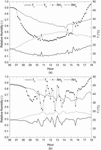
4.4 Hourly variation of the relative humidity of the conditioned environment
Figure 9 shows the behavior of the relative humidity of the conditioned environment $\left(R H_L\right)$ for sunny (a) and cloudy (b) days.
At the beginning of both days, the RHL is high and equals the humidity of the external environment (RHa). From the moment the SCA starts its operation at 7:10 am on a sunny day (Figure 9(a)), the RHL suffers a sharp drop due to the beginning of the dehumidification of the environment, followed by stabilization at a lower level than RHa, with an average value of 49% and an average TL of 21℃. From 03:10 pm, when the TL starts to increase due to the reduction in the cooling capacity of the SCA, the RHL also increases, due to the system decreasing its ability to remove moisture from the air, getting high values till the end of the day. For the cloudy day (Figure 9(b)), RHL remains equal to RHa in the period from 6:00 am to 8:30 am. The SCA starts its operation, causing the RHL to suffer a drop until 9:20 am, from then on oscillating according to the oscillation of the cooling capacity of the SCA, and consequently of the TL, reaching a level 44% minimum at 12:40 pm.
The states of temperature and relative humidity RHL of the conditioned environment, reached during the period of operation of the ACS, for the two days analyzed, can be seen in Figure 10.
Figure 9. Hourly variation of the relative humidity (RH) of the conditioned environment for (a) sunny and (b) cloudy days
Figure 10. Thermal comfort conditions for the indoor environment
For the operation of the system on a sunny day, it appears that only 18 points are within the thermal comfort zone established by ASHRAE [36], which corresponds to 25% of the library's operating time, and for a cloudy day, only 9 points are within the zone demarcated in the diagram, that is, only 12.3% of the time that the occupants would be inside the library, the equipment would be able to maintain adequate comfort conditions.
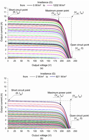
4.5 I-V characteristic curves of the photovoltaic generator
Figure 11 shows the characteristic curves of the photovoltaic generator consisting of 8 KC175GT modules, connected in series, operating on both analyzed days, (a) sunny and (b) cloudy, for all measured irradiance values, obtained from the numerical simulation carried out with the aid of the EES software and based on the work of Villalva et al. [20].
Figure 11. Curve I-V of the PVG for (a) sunny and (b) cloudy days
The variation of the leading electrical parameters of the generator is shown, such as the short circuit current (Isc), the open circuit voltage (Voc), and the voltage and current of the maximum power point (Vm, Im). These parameters are of interest for evaluating the generator's exergy destroyed.
4.6 Exergetic balance for system components (PV-ACS)
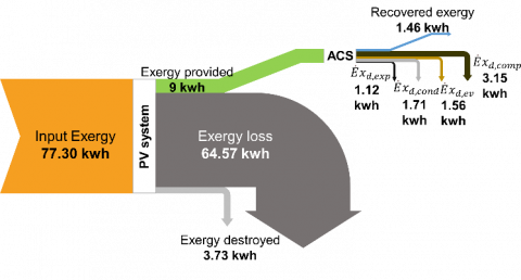
The exergy balance applied to the PV-ACS system, for sunny and cloudy days, respectively, for values integrated during the system operation period is shown in Figures 12 and 13.
It is possible to notice that the photovoltaic system loses most of the input solar exergy, about 64.57 kWh for a sunny day and 27.54 kWh for the cloudy one. This loss occurs during the photovoltaic conversion process, considering the conversion efficiency of the KC175GT modules and the DC-DC and ESC converters.
About 3.73 kWh and 1.36 kWh of exergy are destroyed in the generator on sunny and cloudy days, respectively, because of the internal electrical losses caused by the difference between the product of the open circuit voltage (Voc) and the current of the short circuit (Isc) and the maximum power point (Vm, Im), which intensifies as the solar irradiance increases throughout the day. The destruction of exergy in the generator also occurs due to the heating of the modules as the ambient temperature increases, as shown in Figure 6.
The output exergy of the photovoltaic system is provided for the operation of the ACS. For the sunny day, 9 kWh are supplied, of which 7.54 kWh are destroyed in the components and only 1.46 kWh is considered as the recovered exergy, that is the exergy value of the heat extracted from the conditioned environment. For a cloudy day, the supply by the PV system is 4.18 kWh, of which 3.45 kWh are destroyed and 0.33 kWh are recovered. In summary, the total destroyed exergy of the combined system (PV-ACS) presented values of 11.27 kWh and 5.21 kWh for sunny and cloudy days, respectively.
Figure 12. Exergetic balance for system components (PV-ACS) on a sunny day
Figure 13. Exergetic balance for system components (PV-ACS) on a cloudy day
The percentage value of exergy destruction in each component, over the total exergy destroyed in the combined system (PV-ACS), can be seen in Figure 14.
For the PV system, 33.1% of the exergy is destroyed for a sunny day and 26.10% for a cloudy day. This destruction is mainly due to the heat gain due to the heating of the modules, as well as the internal electrical losses of the system. As the hourly temperature of the cloudy day was lower than that of the sunny day, it implies lower heating of the modules and consequently, less destruction of exergy.
For the compressor, the percentage of exergy destroyed corresponds to 29.2% and 39.9%, for sunny and cloudy days, respectively. Part of the exergy destruction in the compressor is caused, in general, by the friction of the mechanical parts, friction with the refrigerant fluid, and heat dissipation, associated with electrical, mechanical, and isentropic efficiencies [37]. The other part is associated with the supply of electricity by the photovoltaic generator, without promoting the operation of the compressor, at certain times of the day, when the minimum cooling capacity is not reached. For this reason, the percentage of exergy destroyed in the compressor is higher on a cloudy day than on a sunny day.
For the condenser, the destroyed exergy corresponds to 14.70% and 12.10% for sunny and cloudy days, respectively. According to Eq. (38), the irreversibility in the condenser becomes proportional to the increase in mass flow, when the reference temperature (T0) is considered equal to the temperature of the hot environment (TH), which in turn can be equated to the ambient temperature (Ta), causing the exergy destruction in the condenser to be greater for the sunny day, where the mass flux is also greater due to the greater power supplied by the PV system.
Figure 14. Percentage of exergy destroyed in each component concerning the total exergy destroyed in the system (PV-ACS) for sunny (a) and cloudy (b) days
In the evaporator, the exergy destroyed was 13.30% for the system operating on a sunny day and 14.60% for a cloudy day. As the temperature of the external environment increases and the temperature of the conditioned environment decreases, exergy destruction increases proportionally to the temperature difference, this finite difference being a significant source of irreversibilities in heat exchangers [14, 36].
The expansion valve showed a percentage of destroyed exergy of 9.70% and 7.30% for sunny and cloudy days, respectively, with the increase in destruction being proportional to the increase in mass flow and ambient temperature. Although the expansion valve is a component with a dissipative characteristic, for the proposed configuration, it was the component that presented one of the lowest irreversibilities within the combined system.
4.7 Hourly variation of exergy destruction for system components (PV-ACS)
Figure 15 presents the hourly variation of exergy destruction for the combined system (PV-ACS), for sunny (a) and cloudy (b) days, carried out individually in its components, to identify the main sites of exergy destruction throughout the day, from Eqs. (21), (31), (36), (38), (39), and (48), showing the potential for improvement of the system.
The destroyed exergy increases throughout the day for the system components, both for the sunny day (a) and for the cloudy day (b), being greater for the photovoltaic system, followed by the compressor, condenser, evaporator, and expansion valve. For the sunny day, the maximum exergy destruction occurred at 11:40 am, while for the cloudy day, it occurred at 12:40 pm, when the measured irradiance presented the maximum values for the analyzed days.
Figure 15. Hourly variation of exergy destroyed for system components (PV-ACS) for sunny (a) and cloudy (b) days
Increased exergy destruction may be related to greater thermal and mechanical stress on system components. This can shorten the life of these components, leading to a more frequent need for replacement and increasing maintenance costs.
4.8 Variation of exergy destruction for system components (PV-ACS) as a function of measured irradiance increase
The variation of exergy destroyed as a function of measured irradiance is shown in Figure 16.
It is observed that the exergy destruction increases almost linearly for each component of the system, as the irradiance increases. For both analyzed days, the exergy destroyed in the compressor was higher than the other components for irradiance values below 522 W/m². Above this value, the photovoltaic system starts to present the highest rate of exergy destruction.
Figure 16. Variation of exergy destruction for system components (PV-ACS) as a function of irradiance for sunny (a) and cloudy (b) days
4.9 Hourly variation of exergetic efficiency
The hourly variation of exergy efficiency as a function of irradiance variation for systems, PV, ACS, and sys is shown in Figure 17.
It is possible to observe that, for both analyzed days, the ACS and sys efficiencies increase throughout the day, according to the increase in irradiance. The exergy efficiency analysis for the sunny day showed that the ACS reaches a maximum of 19.32% at 11:40 am and the sys of 2.14% at 10:50 am. While for the cloudy day, the maximum values reached were 14.32% at 12:40 pm for ACS and 1.70% at 12:40 am for sys.
Figure 17. Hourly variation of exergetic efficiency for the ACS, the PV, and the combined system for sunny (a) and cloudy (b)
The increase in the efficiencies of both the ACS and the sys is due to the growth of the cooling capacity of the ACS and the difference between the temperatures Ta and TL, which causes an increase of $\dot{X}_{Q_L}$ and, consequently, of the system efficiency. For cloudy days, the exergy efficiency is oscillatory, reaching zero values at times due to the period in which the ACS does not meet the minimum cooling capacity, thus remaining inoperative.
The exergy efficiency of the PV system is reduced throughout the day as there is an increase in the irradiance and temperature of the photovoltaic modules, which causes greater destruction of exergy in the generator. The exergy efficiency of the PV system reaches a minimum value of 11% at 12:50 pm for a sunny day and 11.83% at 12:40 pm for a cloudy day.
4.10 Hourly variation of the COP for the combined system (PV-ACS)
Figure 18 shows the COP hourly variation for the combined system (COPsys), for different evaporating temperatures.
It is possible to see that as the evaporation temperature increases, the COPsys also increase for both days. For a sunny day, COPsys presented the highest value of 0.84 for a Tev of 10℃, at the beginning of the ACS operation, and the lowest value of 0.24 at 12:50 pm for an evaporation temperature of -10℃. While for the cloudy day, COPsys showed an oscillatory behavior, reaching zero values when the system was not operating, with the highest value of 0.72 at 8:30 am, for a Tev of 10℃ and the lowest value of 0.28 at 12:40 pm, for the evaporating temperature of -10℃.
Figure 18. Hourly variation of the coefficient of performance for the combined system (PV-ACS) for different evaporation temperatures on sunny (a) and cloudy (b) days (TL (a)=21℃, TL (b)=24℃)
4.11 Variation of exergetic efficiency of the combined system
The hourly variation of the exergy efficiency of the combined system, for different evaporation temperatures is shown in Figure 19.
The analysis was performed considering the reference temperature equal to the ambient temperature (T0=Ta ), where it is observed that the exergy efficiency of sys increases throughout the day, influenced by the increase in ambient temperature (see Figure 6). According to the simulation, for different evaporation temperatures, it is possible to notice that the exergy efficiency increases correspondingly to the increase in the evaporation temperature, with the highest efficiency values occurring for Tev of 10℃, for both days, with magnitudes 1.97% for a sunny day and 0.60% for a cloudy day.
The results obtained showed notable similarities regarding the behavior of the cooling capacity curves, Coefficient of Performance (COPsys), and exergy efficiency, with the study conducted by Salilih and Birhane [8]. This concordance in the results suggests consistency in the patterns observed in different studies, reinforcing the trends identified in the behavior of the solar cooling system under investigation.
Figure 19. Variation of exergetic efficiency for the combined system (PV-ACS) for different evaporation temperatures on sunny (a) and an a cloudy (b) days (TL (a)=21℃, TL (b)=24℃)
This work proposed an exergetic analysis of an air conditioning system directly coupled to a photovoltaic generator (PV-ACS), without batteries or grid support. The PV-ACS operates according to the natural regulation of solar energy for two days, with different irradiance profiles (sunny and cloudy), following the methodology used by Santos et al. [19] in Belém, the capital of the state of Pará - Brazil.
The air conditioning system requires a minimum input power of approximately 0.30 kW to achieve the minimum cooling capacity, with an irradiance level of 240 W/m² being required in the PVG to generate this power.
On a sunny day, the proposed system can operate above the minimum cooling capacity for approximately nine hours and forty minutes uninterrupted, however, in just 25% of the library operating time, the temperature and relative humidity parameters would be within the zone of comfort established in [36]. As for the cloudy day, the operation takes place above the minimum cooling capacity for five hours and fifty minutes, considering four interruptions due to the low availability of solar resources, which leaves the system inoperative for one hour and forty minutes throughout the day. Under these conditions, the system can keep the environment within the comfort zone for the occupants, for only 12.3% of the library's operating time.
Due to the buoyancy of the system's cooling capacity throughout the day, component design and sizing would need to be carefully calculated to handle daily variations in solar energy availability.
The analysis and simulation of the PV-ACS system showed that the exergy destruction increases throughout the day for the system components, both on sunny and cloudy days, with the photovoltaic system being the most affected, followed by the compressor, condenser, evaporator, and expansion valve, on a sunny day.
The maximum exergy destruction in the photovoltaic system was 3.73 kWh on a sunny day and 1.36 kWh on a cloudy day, corresponding to about 33.1% and 26.10% of the total exergy destroyed in the PV-ACS system on sunny and cloudy days, respectively.
Increased exergy destruction in system components may be related to greater thermal and mechanical stress, which may reduce the lifetime of these components, leading to a more frequent need for replacement and increasing maintenance costs.
For the ACS, the component with the highest exergy destruction was the compressor, with a value of 3.29 kWh on a sunny day and 2.08 kWh on a cloudy day, corresponding to 29.2% and 39.9% of the total exergy destroyed by the combined system, respectively. Part of the exergy destroyed in the compressor occurs when the system cannot reach the minimum cooling capacity but is still powered by the electricity generated by the photovoltaic system.
The component with the lowest exergy loss was the expansion valve, with a maximum destruction of 1.09 kWh on a sunny day and 0.38 kWh on a cloudy day, corresponding to 9.70% and 9.30% of the total exergy destroyed in the combined system on sunny and cloudy days, respectively. Overall, the total exergy destroyed in the combined system (PV-ACS) was 11.27 kWh and 5.21 kWh for both days analyzed.
It was possible to verify that the exergetic efficiency of the ACS and the system increases throughout the day for both analyzed irradiance profiles, due to the increase in cooling capacity and the difference between external and conditioned environment temperatures.
For the photovoltaic system, the exergetic efficiency decreases throughout the day as irradiance and ambient temperature increase, causing an increase in exergy destruction due to electrical losses associated with the photovoltaic module characteristics and PVG heating. It was found that the reduction of the COPsys throughout the day occurs with the increase of irradiance and ambient temperature and that the COPsys increase with the increase of the ACS evaporation temperature.
The study showed that the exergetic efficiency of the combined system increases with the increase in evaporation temperature and ambient temperature, when the ambient temperature is considered as the reference temperature of the dead state, reaching a maximum of 1.97% for a sunny day and 0.60% for a cloudy day.
Although the system simulation has shown that the operation of the ACS can be regulated from the direct coupling to the PV system, without energy storage, the large variations in temperature and relative humidity can lead occupants to discomfort at various times of the day, especially on cloudy days.
Some practical applications of the proposed system may include small or medium-sized houses, where the energy demand for air conditioning is not excessively high. However, the building's energy efficiency and thermal insulation would be crucial factors to optimize the use of available solar energy. In addition, buildings with a low energy load, such as small clinics or offices, can be considered for this system, especially when the air conditioning energy demand is not high. Proper sizing and energy efficiency remain key to ensuring the maximum use of solar energy and system functionality in meeting these diverse needs.
The experimental validation of the proposed system is necessary for further studies, as well as the implementation of control logic that optimizes the operation in different irradiation conditions, to balance the efficient performance of the system and the thermal comfort of the occupants.
Based on the results found in this study, it was possible to evaluate the places in the system where the most significant exergy destruction occurs when the input power for the air conditioning system is variable, according to the availability of solar resources. This information can serve as a subsidy for the improvement, optimization, and development of new components for systems with configurations similar to the one proposed in this study.
Funding: This work was supported by the national research council – CNPq and GEDAE/UFPA.
[1] Bozgeyik, A., Altay, L., Hepbasli, A. (2022). A sub-system design comparison of renewable energy based multi-generation systems: A key review along with illustrative energetic and exergetic analyses of a geothermal energy based system. Sustainable Cities and Society, 82: 103893. https://doi.org/10.1016/j.scs.2022.103893
[2] Hepbasli, A. (2008). A key review on exergetic analysis and assessment of reneable energy resources for a sustainable future. Renewable and Sustainable Energy Reviews, 12(3): 593-661. https://doi.org/10.1016/j.rser.2006.10.001
[3] OECD/IEA. (2013). Transition to Sustainable Buildings—Strategies and Opportunities to 2050, International Energy Agency, Paris, France. https://www.iea.org/reports/transition-to-sustainable-buildings, accessed on Feb. 21, 2023.
[4] Atam, E. (2017). Current software barriers to advanced model-based control design for energy-efficient buildings. Renewable and Sustainable Energy Reviews, 73(8): 1031-1040. https://doi.org/10.1016/j.rser.2017.02.015
[5] Aguilar, H.M.C., Pinho, J.T., Galhardo, M.A.B. (2007). Design of an Efficient Building in Hot and Humid Climate. II Brazilian Congress of Energy Efficiency, Vitória.
[6] Cardoso, L. (2022). Amazônia tem mais de 425 mil famílias sem energia elétrica. Site OECO. https://oeco.org.br/reportagens/amazonia-tem-mais-425-mil-familias-sem-energia-eletrica, accessed on May. 20, 2022.
[7] Kaushik, S.C., Hans, R., Manikandan, S. (2016). Theoretical and experimental investigations on solar photovoltaic driven thermoelectric cooler system for cold storage application. International Journal of Environmental Science and Development, 7(8): 615-620. https://doi.org/10.18178/ijesd.2016.7.8.850
[8] Salilih, E.M., Birhane, Y.T. (2019). Modeling and performance analysis of directly coupled vapor compression solar refrigeration system. Solar Energy, 190: 228-238. https://doi.org/10.1016/j.solener.2019.08.017
[9] Bayrakçi, H.C., Özgür, A.E. (2009). Energy and exergy analysis of vapor compression refrigeration system using pure hydrocarbon refrigerants. International Journal of Energy Research, 33(12): 1070-1075. https://doi.org/10.1002/er.1538
[10] Szargut J., Petela R. (1965). Egzergia (Exergy). Warszawa, WNT.
[11] Szargut, J., Morris, D., Steward, F. (1998) Exergy Analysis of Thermal, Chemical and Metallurgical Processes. New York: Hemisphere Publishing Corporation.
[12] Bilgili, M. (2011). Hourly simulation and performance of solar electric-vapor compression refrigeration system. Solar Energy, 85(11): 2720-2731. https://doi.org/10.1016/j.solener.2011.08.013
[13] Aguilar, F.J., Aledo, S., Quiles, P.V. (2017). Experimental analysis of an air conditioner powered by photovoltaic energy and supported by the grid. Applied Thermal Engineering, 123: 486-497. https://doi.org/10.1016/j.applthermaleng.2017.05.123
[14] Ahamed, J.U., Saidur, R., Masjuki, H.H. (2011). A review on exergy analysis of vapor compression refrigeration system. Renewable and Sustainable Energy Reviews, 15(3): 1593-1600. https://doi.org/10.1016/j.rser.2010.11.039
[15] Anand, S., Tyagi, S.K. (2012). Exergy analysis and experimental study of a vapor compression refrigeration cycle: A technical note. Journal of Thermal Analysis and Calorimetry, 110(2): 961-971. https://doi.org/10.1007/s10973-011-1904-z
[16] Mosaffa, A.H., Farshi, L.G., Ferreira, C.I., Rosen, M.A. (2014). Advanced exergy analysis of an air conditioning system incorporating thermal energy storage. Energy, 77: 945-952. https://doi.org/10.1016/j.energy.2014.10.006
[17] Sogut, M.Z. (2012). Exergetic and environmental assessment of room air conditioners in Turkish market. Energy, 46(1): 32-41. https://doi.org/10.1016/j.energy.2012.06.065
[18] Aman, J., Ting, D.K., Henshaw, P. (2014). Residential solar air conditioning: Energy and exergy analyses of an ammonia–water absorption cooling system. Applied Thermal Engineering, 62(2): 424-432. https://doi.org/10.1016/j.applthermaleng.2013.10.006
[19] Santos, E.C., Macêdo, E.N., Galhardo, M.A., Costa, T.O., Costa, A.F.P., Brito, A.U., Oliveira, L.G.M., Macêdo, W.N. (2021). Analysis of the behavior of an air conditioning system based on the solar energy natural regulation in Amazonian climatic conditions. Journal of Solar Energy Engineering, 143(3): 031001. https://doi.org/10.1115/1.4048275
[20] Villalva, M., Gazoli, J., Filho, E. (2009). Comprehensive approach to modeling and simulation of photovoltaic arrays. IEEE Transactions on Power Electronics, 24(5): 1198-1208. https://doi.org/10.1109/TPEL.2009.2013862
[21] Bana, S., Saini, R.P. (2016). Identification of unknown parameters of a single diode photovoltaic model using particle swarm optimization with binary constraints. Renewable Energy, 101: 1299-1310. https://doi.org/10.1016/j.renene.2016.10.010
[22] Carrero, C., Amador, J., Arnaltes, S. (2007). A single procedure for helping PV designers to select silicon PV modules and evaluate the loss resistances. Renewable Energy, 32(15): 2579-2589. https://doi.org/10.1016/j.renene.2007.01.001
[23] Odeh, N., Grassie, T., Henderson, D., Muneer, T. (2006). Modelling of flow rate in a photovoltaic-driven roof slate-based solar ventilation air preheating system. Energy Conversion and Management, 47(7-8): 909-925. https://doi.org/10.1016/j.enconman.2005.06.005
[24] Pinho, J.T., Galdino, M.A. (2014). Manual de engenharia para sistemas fotovoltaicos. Rio de Janeiro, 1: 47-499.
[25] Rawat, R., Kaushik, S.C., Lamba, R. (2016). A review on modeling, design methodology and size optimization of photovoltaic based water pumping, standalone and grid connected system. Renewable and Sustainable Energy Reviews, 57: 1506-1519. https://doi.org/10.1016/j.rser.2015.12.228
[26] Bayrak, F., Ertürk, G., Oztop, H.F. (2017). Effects of partial shading on energy and exergy efficiencies for photovoltaic panels. Journal of Cleaner Production, 164: 58-69. https://doi.org/10.1016/j.jclepro.2017.06.108
[27] Petela, R. (2008). An approach to the exergy analysis of photosynthesis. Solar Energy, 82(4): 311-328. https://doi.org/10.1016/j.solener.2007.09.002
[28] Joshi, A.S., Dincer, I., Reddy, B.V. (2009). Thermodynamic assessment of photovoltaic systems. Solar Energy, 83(8): 1139-1149. https://doi.org/10.1016/j.solener.2009.01.011
[29] Pandey, A.K., Tyagi, V.V., Tyagi, S.K. (2013). Exergetic analysis and parametric study of multi-crystalline solar photovoltaic system at a typical climatic zone. Clean Technologies and Environmental Policy, 15(2): 333-343. https://doi.org/10.1007/s10098-012-0528-8
[30] Tiwari, G.N. (2002). Fundamentals, design, modeling and applications. Solar Energy, 279-309.
[31] Sahin, A., Dincer, I., Rosen, M.A. (2005). Thermodynamic analysis of wind energy. International Journal of Energy Research, 30(8): 553-566. https://doi.org/10.1002/er.1163
[32] Koroneos, C., Tsarouhis, M. (2012). Exergy analysis and life cycle assessment of solar heating and cooling systems in the building environment. Journal of Cleaner Production, 32: 52-60. https://doi.org/10.1016/j.jclepro.2012.03.012
[33] Özgoren, M., Erdoğ an, K., Kahraman, A., Solmaz, O., Köse, F. (2010). Calculation of dynamic cooling load capacity of a building air-conditioning powered by wind or solar energy. International Aegean Energy Symposium and Exhibition (IEESE-5), Denizli, June, pp. 27-30.
[34] Çengel, Y., Boles, M. (2015). Thermodynamics: An Engineering Approach, 8th Edition. McGraw-Hill Book Company, New York.
[35] Wang, S.K. (2000). Handbook of Air Conditioning and Refrigeration (Vol. 2). Load Calculations, New York: McGraw-Hill, pp. 6.1 - 6.55.
[36] ASHRAE STANDARD 55. (2017). Thermal environmental conditions for human occupancy. Atlanta, Georgia: American Society of Heating Refrigerating and Air-Conditioning Engineers.
[37] Kotas, T.J. (2013). The Exergy Method of Thermal Plant Analysis. Elsevier.