Matteo Malavasi*![]() | Luca Cattani
| Luca Cattani![]() | Alessandro Benelli
| Alessandro Benelli![]() | Luca Pagliarini
| Luca Pagliarini![]() | Fabio Bozzoli
| Fabio Bozzoli![]()
(This article is part of the Special Issue 8th AIGE/IIETA International Conference and 18th AIGE Conference)
© 2023 IIETA. This article is published by IIETA and is licensed under the CC BY 4.0 license (http://creativecommons.org/licenses/by/4.0/).
OPEN ACCESS
The food industry consumes a substantial amount of energy with a large portion dedicated to product heat treatments. Thus, enhancing the efficiency of thermal operations could significantly decrease energy demand, reduce costs, and mitigate pollution in this sector. This is particularly applicable in vinification, where the grape must's temperature is crucial to the final wine quality. In this process, the energy required for fermentative thermostating constitutes a majority of the total energy expenditure. Furthermore, the thermal management of fermenting grape must is influenced by the heat released during the fermentation process. Therefore, understanding the precise distribution of heat release during fermentation could considerably improve the energy efficiency of this production. This study proposes and validates a methodology to achieve this objective. The approach is based on the inverse problem technique, which utilizes temperature measurements of the fermenting product. The validation of this technique shows promising results, indicating the potential applicability of our proposed method.
fermentation heat, wine industry, inverse problem
In the food industry, approximately 75% of the required energy is expended on heat transfer operations. Together with the tobacco industry, this accounts for 9.8% of the total energy consumed by the manufacturing sector in the European Union [1].
Consequently, enhancing the efficiency and efficacy of these operations is pivotal in reducing energy consumption and associated pollution in this sector [2]. This is evident in the wine-making industry, where the temperature of the fermenting substrate during oenological fermentation processes is of fundamental importance. The temperature can directly activate and regulate the microbial kinetics of the yeast [3-5], which is responsible for converting sugar into ethanol [6], thus impacting the fermentation kinetics [7]. Furthermore, temperature can regulate yeast metabolism, determining the production of primary and secondary molecular compounds during the process. These compounds ultimately influence the nature and amount of volatile aromatic molecules synthesized [8], consequently affecting the organoleptic quality of the final product.
The complexity of managing this process arises from the exothermic character generally exhibited by alcoholic fermentation reactions. These reactions generate significant heat (approximately 106.3 kJ per mole of glucose in the grape must [7]), which is partially absorbed by the wort during the process. This phenomenon could elevate the grape must's temperature, affecting the metabolism of the yeasts involved in fermentation, or even reaching temperatures that could be lethal to them [7].
The rise in temperature is contingent on the applied fermentation conditions. This variability further complicates thermal management in fermenting tanks, particularly in maintaining the correct fermentation temperature within the grape juice. Therefore, accurate knowledge of the net heat generated by fermentation is crucial for better design of fermenter tanks and their thermal control systems, potentially leading to energy improvements in the entire production process.
Several authors have proposed models to estimate the heat developed by alcoholic fermentation. Wiliams [9] proposed a correlation of the heat developed by fermentation as a function of the must's sugar concentration. Colombiè et al. [6] proposed an estimation model of the heat produced by oenological fermentation, based on correlations and validated with experimental data. Lòpez and Secanell [10] proposed and experimentally validated a mathematical model for estimating the kinetics of heat production during fermentation.
However, several factors contribute to the heterogeneity of the heat release during fermentation and the temperature variation of the must inside the tank. These include the must's physic-chemical properties (such as glucose concentration), initial fermentation temperature, fermentation kinetics, fluid-dynamic conditions in the tanks due to the mechanical action of ascending CO2 bubbles produced during the process, and possible temperature gradients (especially in the case of red wine-making processes) [6]. Therefore, estimating the heat produced during fermentation is complicated. The specific models available in the scientific literature are strictly related to validation conditions and may not be suitable for any specific alcoholic fermentation circumstances adopted by different wine producers.
With this in mind, the focus should be on developing and validating a heat flux estimation methodology, rather than estimating a specific case study. To this end, an estimation approach for determining the heat release rate during fermentation in wine making processes has been developed. This procedure is based on an inverse problem approach: by measuring the evolution of the grape must's temperature during fermentation (effect), the heat generated by the process (cause) is estimated.
The developed model is proposed as a practical tool for accurately determining the heat release curve of the applied alcoholic fermentation, overcoming the problem of poor adaptability to variations in fermentation conditions of analytical models. Specifically, the proposed procedure enables the estimation of the specific heat release curve of the fermentation of interest, obtained from experimental in-field measurements of the must temperature evolution during the studied process.
In doing so, the difficulty of adapting the analytical model to the numerous different fermentation conditions used by various producers is eliminated. Therefore, this model is expected to provide accurate estimations for the cases where it will be applied, and to be characterised by high applicability due to its ease of implementation in user-friendly software for manufacturers. This approach could also simplify the thermal sizing of innovative temperature control systems (alternatives to the classic cooling jacket used in stainless steel fermentation tanks in wineries), such as heat pipes, which can be easily applied to the food industry, like the coffee one [11].
2.1 The inverse problem approach
In this inverse problem, the power generated inside the product was the object to be estimated while the temperatures of the grape must under fermentation represents the input dataset. The description of the estimation procedure starts with the modelling of the direct heat-transfer problem of a tank containing the must under fermentation, proceeds with the solution of the inverse problem by applying the Tikhonov regularization method and concludes with the estimation of the generated power over the time of fermentation. The energy balance equation of the system can be written as follow:
$\begin{gathered}\dot{Q}_f(t)=m c_p \frac{d T}{d t}+h A\left(T(t)-T_e(t)\right) \\ T(t=0)=T_i\end{gathered}$ (1)
where, $\dot{Q}_f[\mathrm{~W}]$ is the power input generated inside the product, $T\left[{ }^{\circ} \mathrm{C}\right]$ is the measured average temperature of the product, $T_e$ $\left[{ }^{\circ} \mathrm{C}\right]$ is the environment temperature, $\tau[\mathrm{s}]$ is the time, $h\left[\mathrm{~W} \mathrm{~m}^{-}\right.$ $\left.2^{\circ} \mathrm{C}^{-1}\right]$ is the convective heat transfer on the external side of the $\operatorname{tank}, A\left[m^2\right]$ is the external surface of the tank. Regarding the variables $m$ (mass) and $c_p$ (specific heat), they refer to the system composed by the union of the tank and of the water.
If for the direct problem of this situation, the value of $\dot{Q}_f$ is known (cause) while the value of $d T$ (effect) is unknown, for the inverse problem the condition is the exact opposite: $d T$ (effect) is experimentally measured while $\dot{Q}_f$ (cause) is unknown.
$\dot{Q}_f(t)-h A\left(T(t)-T_e(t)\right)=m c_p \frac{d T}{d t}=\dot{Q}_{a c c}$ (2)
Introducing the term $\dot{Q}_{a c c}$ [W] that corresponds to the net heat input power accumulated by the product inside the tank during the test.
In this case, $\dot{Q}_{a c c}$ represent the terms that is estimated and, for this reason, as suggested by Beck et al. [12] and Dennis et al. [13], because the inverse problem is linear with respect to it, the problem can be written in the discrete domain as follows:
$T=\dot{Q}_{a c c} X+T_{\dot{Q}_{a c c}=0}$ (3)
where, $X$ is the sensitivity matrix and $T_{\dot{Q}_{a c c}=0}$ is a constant term that correspond to the average temperature of the product in case of null $\dot{Q}_{a c c}$.
$X$ is the sensitivity matrix of $N \times N$ dimension and the vector $T_{\dot{Q}_{a c c}=0}$, of dimension $N, N$ is the total number of acquisitions, can be explicated as follow:
$X=\left[\begin{array}{ccccc}\frac{\Delta t}{m c_p} & 0 & 0 & \ldots & 0 \\ \frac{\Delta t}{m c_p} & \frac{\Delta t}{m c_p} & 0 & \ldots & 0 \\ \vdots & \vdots & \vdots & \cdots & 0 \\ \frac{\Delta t}{m c_p} & \frac{\Delta t}{m c_p} & \frac{\Delta t}{m c_p} & \cdots & \frac{\Delta t}{m c_p}\end{array}\right], T_{\dot{Q}_{a c c}=0}=\left[\begin{array}{c}T_i \\ T_i \\ \vdots \\ T_i\end{array}\right]$ (4)
In the inverse formulation, the computed temperature distribution T is forced to match the experimental temperature distribution Y, by tuning the value of $\dot{Q}_{a c c}$. The matching of the two temperature distributions (the computed and the experimentally one) could be easily performed under a least square approach. However, the ill-posed nature of the problem, makes the least square solution dominated by noise, and for this reason the Tikhonov regularization method is adopted in the present work as regularization technique; this approach has been successfully used in the inverse heat-transfer literature [14] making possible to reformulate the original problem as a well-posed problem. In this case, it consists in the minimization of the objective function here reported:
$\begin{gathered}J\left(\dot{Q}_{a c c}\right)=\left\|Y-\dot{Q}_{a c c} X-T_{\dot{Q}_{a c c}=0}\right\|_2^2+ \\ \lambda^2\left\|L \dot{Q}_{a c c}\right\|_2^2, \dot{Q}_f>0\end{gathered}$ (5)
where, $\|\cdot\|_2^2$ stands for the square of the 2-norm, λ is the regularization parameter, L is the derivative operator and T is the average temperature of the product measured by imposing a given $\dot{Q}_{a c c}$. Since the choice of a proper regularisation parameter requires a good balance between the size of the residual norm and the size of the solution norm (semi norm), the L-curve method proposed by Hansen and O’Leary [15] was used.
2.2 Validation of the model with synthetic data
Before applying the estimation model to experimental measurements, it was validated using a synthetic dataset. To this purpose, a synthetic heat curve release (see Figure 1), representing the non-constant kinetics of the yeast throughout the fermentation time was used to obtain the evolution of the substrate temperature T. The curve considered represents the typical behaviour of the kinetics of the yeast involved in oenological processes, specifically for the case of the fermentation of 100 l of grape juice inside a fermenter tank [9], [16]. The concentration of glucose in a grape must for vinification can reach 1.7 mol/l and, from the stochiometric ideal case, each mole of glucose fermented by the yeast can release heat up to about 100 kJ. Moreover, it is possible to state that only in the first two days of fermentation, i.e., those where the metabolic activities of the yeast are at the maximum level, the maximum amount of heat power (in this case about 1 W/l) is released in the grape must. However, over the course of a week-long fermentation, it is possible to say that this value of power released per litre of grape must represents the maximum peak attainable by the process, since the metabolic kinetics of the yeast are not constant throughout the fermentation time, but they are mainly concentrated in its first few days: most of the heat is released in 48-72 hours (~80-90%), while for the rest of the fermentation time the power generated is approximately 20% of the initial peak [16].
Figure 1. Synthetic heat curve
For this application, the starting temperature of the fermentation substrate was considered about 28℃ and the container was considered perfectly insulated from the environment. The variation of the temperature of the product over the time, T, was computed reformulating the definition of the direct problem reported in Eq. (1) as follow:
$\frac{\dot{Q}_f(t) d t}{m c_p}+T(t-d t)=T(t)$ (6)
$T(t=0)=28^{\circ} \mathrm{C}$ (7)
where, $\dot{Q}_f$ [W] is the known heat power released by the fermentation, dt [s] is the time between acquisitions, cp [Jkg-1K-1] is the specific heat of the system, m [kg] is the mass of the system and T [℃] is the temperature of the product.
The distribution of the computed product temperature T, was then spoiled with random noise for simulating a real experimental dataset:
$\mathrm{T}_{\text {noise }}=\mathrm{T}+\zeta \epsilon$ (8)
where, ϵ is a random Gaussian variable with zero mean and unit variance and ζ is the temperature noise level; in the present case was considered equal to 0.1℃ that corresponds to the measurement uncertainty of the thermocouples. The distribution of the noisy temperature is reported in Figure 2.
Finally, this dataset was used for the estimation of the input power released by the fermentation $\dot{Q}_f$ using the inverse problem solution approach reported in Eq. (5).
Figure 2. Distribution of noisy temperature used for the validation
Figure 3. Comparison between the estimated heat curve release and the synthetic one
In Figure 3 the comparison between the estimated heat curve release and the synthetic one is reported. It is possible to see that a very good accordance is shown between the two distributions, highlighting the good performances of the model in estimating the heat released during fermenting phenomena. For this reason, it is possible to consider the model validated.
To confirm this, in Figure 4 the evolution of the residual (ResQ) between the and the Q estimated ($Q_{\text {estimated }, i}\,\,\,$) and the synthetic one ($Q_{\text {estimated }, i}\,\,\,$), calculated as follow:
$\operatorname{Res}_{Q, i}=Q_{\text {estimated }, i}-Q_{\text {synthetic }, i}$ (9)
with i corresponding to the ith acquisition.
It is possible to see that it reaches a value of -5.5 W in the first minutes of estimation, while, for the rest of the time, it keeps a value hovering around ±1.5 W, confirming another time the success of the validation process with synthetic data.
Figure 4. Residual (ResQ) between the Q synthetic and the estimated one
2.3 Validation of the procedure with experimental data
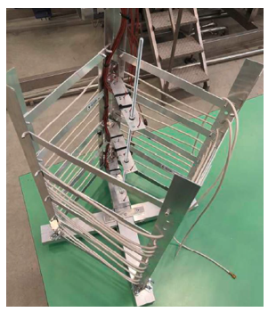
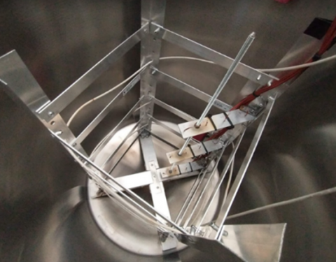
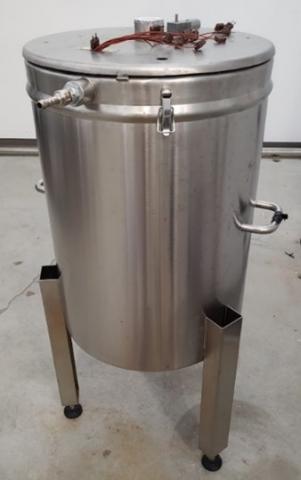
For experimental validation step, a tank in AISI 316L with an internal volume of 100 l was realized. The heat generation during fermentation was simulated using 2 immersion thermoelectric resistances: one of 40 W and the other one of 100 W. In this way it was possible to reproduce a change in the power generation during the tests, simulating the change in the microbial kinetics that usually occurs during an alcoholic fermentation. To simplify the model, water was used as substitute of the fermenting substrate as grape must is principally composed of it. The wire thermoelectric resistances were spirally disposed inside the tank using a mechanical support structure specially realized in aluminum to have the most possible uniform heat generation inside the tank (Figure 5(a)).
(a)
(b)
(c)
(d)
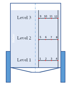
Figure 5. Measurements setup used for experimental validation: a) mechanical support for the thermal resistance and for the thermocouples; b) mechanical support placed inside the fermenter tank c) schematic representation of the tank, the 100 l of water inside it and the placement of the thermocouples and d) external view of the fermenter tank with the thermocouples inserted
The variable input power, reproducing the non-constant kinetics of the yeast involved described in paragraph 2.2, was performed considering 2 values for the initial heat peak and for each, 2 time intervals. In specific, the power inputs of the peak were: the theoretical one of 100 W and 140 W (+40%), while the time durations of every peak were: 1 h and 2 h. The input power for the remaining time of the fermentation was kept at about 40W. The total time of every single simulation of fermentation was of 3.5 h, excluding the initial period when the input power was not present.
In the tests performed for the validation, the temperature of the product inside the tank was acquired in 12 different positions (Figure 5(b)) by means of 12 T-type thermocouples, at 4 radial distances for 3 axial coordinates. The three height levels were spaced 150 mm one from the other with the first level about 150 mm from the bottom of the tank. For each level, the thermocouples were located at the radial distances of 6 cm, 115 mm, 170 mm, and 225 mm from the longitudinal axis, respectively. Thermocouples were held in position inside the tank using the same mechanical support used for the thermal resistance (Figure 5(a) and 5(b)). Finally, the ambient air temperature was measured with 3 additional T-type thermocouples placed in proximity of the tank. Every temperature was acquired every 3s.
Moreover, for improving the estimation model, an in-situ estimation of h A and m cp expressed in Eq. (2) was performed.
For calculating these two parameters, 2 additional tests were executed. In the first test, the 100 l of water inside the tank were heated, starting from room temperature, by means of a 100 W wire immersion thermal resistance while, in the second test, the water was cooled back to room temperature by natural convection. During both tests, the water and the ambient temperatures were acquired with the system described above.
The energy balance equations describing the cooling and heating tests can be written as reported in Eq. (10) and Eq. (11), respectively.
$m c_p \frac{d T_c}{d t_c}=h A\left(T_c-T_e\right)$ (10)
$m c_p \frac{d T_h}{d t_h}=\dot{Q}_{e l}-h A\left(T_h-T_e\right)$ (11)
where, Tc is the temperature of the product in the cooling test while Th in the heating test, Te is the temperature of the environment and $\dot{Q}_{e l}$ is the input power of the wire resistance if it is present.
To isolate the two unknowns h∙A and m∙cp, Eq. (11) can be rewritten as follow:
$\frac{m c_p}{h A}=\left(T_c-T_e\right) \frac{d t_c}{d T_c}$ (12)
Substituting it in Eq. (12), it is possible to obtain:
$h A=\frac{\dot{Q}_{e l}}{\left(T_c-T_e\right) \frac{d t_c}{d T_c} \frac{d T_h}{d t_h}+\left(T_h-T_e\right)}$ (13)
Once $h A$ was estimated, it was possible also to calculate the term $m c_p$. In specific, $m c_p$ is about $4.5 \cdot 10^5 \mathrm{~J} / \mathrm{K}$, while $h A$ is $3.39^{\circ} \mathrm{C} / \mathrm{W}$.
Finally, using $h A$ parameter, and starting from the estimated value $\dot{Q}_{a c c}$, it was possible to calculate the value of the power generated by the fermentation $\dot{Q}_f(t)$, as follow:
$\dot{Q}_f(t)=h A\left(T(t)-T_e(t)\right)+\dot{Q}_{a c c}$ (14)
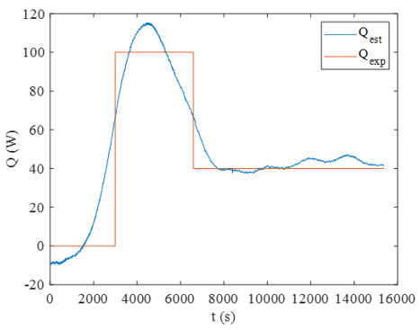
Observing the comparison of the real input power curve and the estimated one in function of the time for the two tests carried out with peak input power of 100 W (Figure 6(a) and 6(b)), it is possible to state that the estimation model can satisfactorily reconstruct the trend of the curve of the input power supplied to the product during the simulation of the fermentation process. It can be observed that the course and slopes of the curve are satisfactorily reproduced both at the beginning and at the end of the process. To better describe the behaviour of the estimation curve, the mean percentage error of the estimation $\overline{\operatorname{Err}_Q}$ is considered and it is calculated as follow,
$\overline{E r r_Q}=\frac{\sum_{i=1}^n \frac{Q_{\text {real }, i}\,\,\,-Q_{\text {estimated }, i}}{Q_{\text {real }, i}}}{N} \%$, (15)
with N that is the total number of acquisitions. From the analysis of this parameter, it is possible to note that the highest value for $\overline{\operatorname{Err}_Q}$, of about 18.06% (Table 1), is reached when the peak input power duration time was of 2 h, while for the test with peak input power duration time of 1 h the value of $\overline{E r r_Q}$ reached 9.82%. These values confirm another time that the model is able to reproduce the behaviour of the curve of power generated during the fermentation. Moreover, analysing and matching these values with Figure 6, it is possible to notice that the major discrepancy between the curves of the estimated input power and the experimental ones occurs at the moments of power switching for each test and it is possible to affirm that the calculated error at these moments mainly contributes to increase the value of $\overline{E r r_Q}$ for every test.
(a)
(b)
(c)
(d)
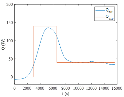
Figure 6. Comparison between the real input power and the estimated one for the case: a) 100 W – 1 h; b) 100 W – 2 h; c) 140 W – 1 h; d) 140 W – 2 h
Table 1. $\overline{\operatorname{Err}_Q}$ of every test
|
Peak input Power [W] |
100 |
140 |
||
|
Duration Time [h] |
1 |
2 |
1 |
2 |
|
$\overline{\operatorname{Err}_Q}$[%] |
9.82 |
18.06 |
19.95 |
15.34 |
However, if we consider a real fermentation process, the heat power generated inside the grape must generally does not change so sharply, so the need to estimate power input in such a sharp change in input power could be considered not necessary for the application of this model and the error of estimation in that phase could be considered negligible. In this case, the estimation error $\overline{\operatorname{Err}_Q}$ would be further reduced, strengthening the validation of the model. Moreover, in a real case of fermentation, the amount of heat released would be lower than the stochiometric theoretically calculated one.
However, the authors chose these validation conditions as they represent the most challenging ones for the estimation system. Nevertheless, the model proved to be able to estimate the power generated during fermentation with good accuracy in the tests with an input peak power of 100 W.
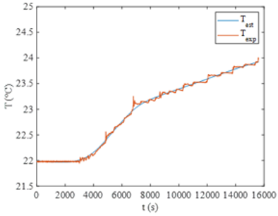
Observing the comparison of the real input power curve and the estimated one in function of the time, also for the tests with the peak input power of 140 W in Figure 6, it is possible to state that the model was able to estimate quite accurately the trend of the power input curve inside the product during the fermentation simulation. However, it seems that an increased difference between the peak and the rest of the input power during the test, quite increased the error in estimation. In specific, the highest value of $\overline{\operatorname{Err}_Q}$ was of 19.95% (Table 1) and it was reached in the test with the duration time of the peak input power of 1 h, while for the tests with the duration of the peaks input power of 2 h, it was 15.34%. However, also in these cases the major discrepancy between the estimated and real input power curves occurs at the moments of the input power switches. To confirm the goodness of the model developed, in Figure 7, it is possible to observe the comparison between the average experimental temperature of the product inside the tank (Texp), measured during the tests, and the simulated temperature (Test) obtained by solving the direct problem using the power estimated adopting the here proposed procedure. It is possible to observe that the simulated temperature perfectly reproduces the real one.
(a)
(b)
(c)
(d)
Figure 7. Comparison between the average experimental temperature of the product inside the tank and the estimated temperature obtained by solving the direct problem using the estimated input power for the case: (a) 100 W – 1 h; (b) 100 W – 2 h; (c) 140 W – 1 h; (d) 140 W – 2 h
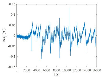
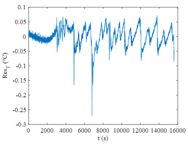
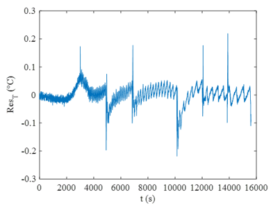
This behaviour is confirmed in Figure 8 by the distribution of the residual $\left(\operatorname{Res}_T\right)$ between the measured temperature (Texp) and the estimated one (Test), reconstructed using the estimated heat released curve, calculated as follow:
$\operatorname{Res}_T=T_{\text {exp }}-T_{e s t}$ (16)
It is possible to observe that the maximum difference of about -0.27℃ is reached in the test with input peak of 140W for 60 min, while for the rest of the time the $\operatorname{Res}_T$ value oscillates in the range -0.2℃–0.2℃ for all the tests.
Finally, it is possible to consider also the maximum value of the percentage error of estimation, calculated as follow:
$\operatorname{Err}_T=\frac{\left|\operatorname{Res}_{T, i}\right|}{T_{\text {exp }, i}} \%$ (17)
where, $\operatorname{Res}_{T, i}$ is the residual calculated as reported in Eq. (16), with i corresponding to the ith acquisition. Observing it, it is possible to see that it reaches 1.15% in the case with a peak power input of 140 W and duration of 1 h, highlighting another time the validation of the procedure developed.
(a)
(b)
(c)
(d)
Figure 8. $\operatorname{Res}_{\mathrm{T}}$ for the case: (a) 100 W – 1 h; (b) 100 W – 2 h; (c) 140 W – 1 h; (d) 140 W – 2 h
A model for estimating the heat release curve during winemaking fermentation process has been developed and validated in two steps: with synthetic data and with experimental data. During the experimental validation, the model was put under stressing condition of fermentation: a simulation of the non-constant kinetics of the yeast involved was performed. In specific, the model was validated simulating 4 different alcoholic fermentation situations in a fermenter tank of 100 l. Since the heat release is concentrated at the beginning of the fermentation process, a peak input power in the product was considered at the initial part of any tests: 2 values were selected for the initial peak of heat input power (100 W and 140 W) and for each, 2 duration times (1 h and 2 h). The results shown that the model satisfactorily reproduces the general trend of the power generated inside the product, both for tests with an initial peak of 100 W and those with an initial peak of 140 W. This result is also confirmed by the $\overline{\operatorname{Err}_Q}$ values even if the model loses its efficiency and accuracy in the proximity of sudden changes in generated power. However, such a sharp change of the input power is uncommon during fermentation because the changes in microbial kinetics and heat generation are usually gradual and, for this reason, this type of error could be considered negligible in this kind of estimation.
Moreover, the good performances of the model are confirmed also by the comparison between the average experimental temperature of the product inside the tank and the simulated one obtained by solving the direct problem with the estimated input power. For the temperature comparison a maximum percentage error ErrT of 1.15% is reached. In view of the results achieved, it is possible to consider the model validated. A future step for this work will be to apply the model to a real case of alcoholic fermentation to refine it and make it a complete tool at the service of wine producers. It is possible to conclude that this method could represent a very useful tool for the estimation of the heat release curve during wine making processes, especially for the cases in which a high precision on the temperature control of the grape must is required during the entire process and, consequently, the knowledge of the heat to be removed from the product in any instant of the fermentation phase is a fundamental information. Moreover, this tool could represent a very effective instrument for the optimization from the energetic point of view, of the thermal control system on the fermentation tanks. Indeed, knowing the amount of heat to be absorbed and knowing the cellar conditions, it could be easier to realized passive or semi-passive system of temperature control for this phase, reducing or even nulling the energetic demand for the management of the temperature of the substrate. In addition, since the model is based on a real dataset obtained directly from one case of fermentation, the heat release curve obtained is specific for the producer case studied. Moreover, performing a small-scale fermentation in the desired cellar condition, the producer will be able to obtain dedicated information about the heat release curve of its personal process of fermentation, limiting the waste of the raw material and the resources. Concluding, a future step that authors would like to fulfil, will be the application and validation of the model in real scale and its application of the model to a real case of fermentation in a wine cellar, to allow the estimation of a real production case.
A special thanks is for Fabiola Conicella, UNIPR Food Science Technologies student, that helped the Authors in experimental test and dataset elaboration.
|
A |
Surface, m2 |
|
cp |
specific heat, J. kg-1. K-1 |
|
h |
Convective heat transfer coefficient W.m-1. K-2 |
|
m |
mass, kg |
|
N |
Number of tests |
|
$\dot{Q}$ |
Power, W |
|
T |
Temperature, ℃ |
|
t |
Time, s |
|
Subscripts |
|
|
acc |
accumulated |
|
c |
cooling |
|
h |
heating |
|
e |
environment |
|
el |
electric |
|
exp |
experimental |
|
ext, estimated |
estimated |
|
f |
fermentation |
|
i |
instant of acquisition |
|
noise |
dataset with noise |
|
p |
product |
|
real |
real |
|
T |
Temperature |
[1] Eurostat. (2013). Final Energy Consumption by Industry. URL: https://ec.europa.eu/eurostat.
[2] Wang, L. (2014). Energy efficiency technologies for sustainable food processing. Energy Efficiency, 7(5): 791-810. https://doi.org/10.1007/s12053-014-9256-8
[3] Torija, M.J., Beltran, G., Novo, M., Poblet, M., Guillamón, J.M., Mas, A., Rozès, N. (2003). Effects of fermentation temperature and Saccharomyces species on the cell fatty acid composition and presence of volatile compounds in wine. International Journal of Food Microbiology, 85(2-1): 127-136. https://doi.org/10.1016/S0168-1605(02)00506-8
[4] Masneuf-Pomarède, I., Mansour, C., Murat, M.L., Tominaga, T., Dubourdieu, D. (2006). Influence of fermentation temperature on volatile thiols concentrations in Sauvignon blanc wines. International Journal of Food Microbiology, 108(3): 385-390. https://doi.org/10.1016/j.ijfoodmicro.2006.01.001
[5] Rollero, S., Bloem, A., Camarasa, C., Sanchez, I., Ortiz-Julien, A., Sablayrolles, J.M., Dequin, S., Mouret, J.R. (2015). Combined effects of nutrients and temperature on the production of fermentative aromas by Saccharomyces cerevisiae during wine fermentation. Applied Microbiology and Biotechnology, 99(5): 2291-2304. https://doi.org/10.1007/s00253-014-6210-9
[6] Colombié, S., Malherbe, S., Sablayrolles, J.M. (2007). Modeling of heat transfer in tanks during wine-making fermentation. Food Control, 18(8): 953-960. https://doi.org/10.1016/j.foodcont.2006.05.016
[7] Molina, A.M., Swiegers, J.H., Varela, C., Pretorius, I.S., Agosin, E. (2007). Influence of wine fermentation temperature on the synthesis of yeast-derived volatile aroma compounds. Applied Microbiology and Biotechnology, 77: 675-687. https://doi.org/10.1007/s00253-007-1194-3
[8] Torija, M.J., Rozes, N., Poblet, M., Guillamón, J.M., Mas, A. (2003). Effects of fermentation temperature on the strain population of Saccharomyces cerevisiae. International Journal of Food Microbiology, 80(1): 47-53. https://doi.org/10.1016/S0168-1605(02)00144-7
[9] Williams, L.A. (1982). Heat release in alcoholic fermentation: a critical reappraisal. American Journal of Enology and Viticulture, 33(3): 149-153. https://doi.org/10.5344/ajev.1982.33.3.149
[10] López, A., Secanell, P. (1992). A simple mathematical empirical model for estimating the rate of heat generation during fermentation in white-wine making. International Journal of Refrigeration, 15(5): 276-280. https://doi.org/10.1016/0140-7007(92)90042-S
[11] Pipatpaiboon, N., Parametthanuwat, T., Bhuwakietkumjohn, N., Rittidech, S., Sichamnan, S. (2022). Applications of heart shaped glass spoon loop oscillating heat pipe (HSGS/LOHP) for making coffee stirrer. International Journal of Heat and Technology, 40(1): 258-266. https://doi.org/10.18280/ijht.400130
[12] Beck, J.V., Blackwell, B., Clair Jr, C.R.S. (1985). Inverse Heat Conduction: Ill-Posed Problems. James Beck, 137-157, 179-180, 198-211.
[13] Dennis, B.H., Dulikravich, G.S. (1999). Simultaneous determination of temperatures, heat fluxes, deformations, and tractions on inaccessible boundaries. ASME Journal of Heat and Mass Transfer, 121(3): 537-545. https://doi.org/10.1115/1.2826014
[14] Bozzoli, F., Cattani, L., Rainieri, S., Bazán, F.S.V., Borges, L.S. (2014). Estimation of the local heat-transfer coefficient in the laminar flow regime in coiled tubes by the Tikhonov regularisation method. International Journal of Heat and Mass Transfer, 72: 352-361. https://doi.org/10.1016/j.ijheatmasstransfer.2014.01.019
[15] Hansen, P.C., O’Leary, D.P. (1993). The use of the L-curve in the regularization of discrete ill-posed problems. SIAM Journal on Scientific Computing, 14(6): 1487-1503. https://doi.org/10.1137/0914086
[16] Ribéreau, G.P., Dubourdieu, D., Donéche, B., Lonvaud, A. (2007). The microbiology of wine and vinifications. Handbook of Enology, 1: 1-71. https://doi.org/10.1002/9781119588320