Maomao Liu![]() | Liping Wu*
| Liping Wu*![]() | Kaifeng Wu
| Kaifeng Wu![]() | Jingpeng Li
| Jingpeng Li![]()
© 2023 IIETA. This article is published by IIETA and is licensed under the CC BY 4.0 license (http://creativecommons.org/licenses/by/4.0/).
OPEN ACCESS
With the continuous development of the Internet of Things (IoT) and new energy utilization technology, the energy management and monitoring mode has undergone fundamental changes. Design and development of remote real-time monitoring and management system for multi-energy heat collection has certain theoretical and practical application value. The existing remote temperature control model fully considers neither the impact of multi-energy collaborative heat collection on remote temperature control strategy, nor the interactions among multiple objective factors, such as climate and location. Therefore, this paper studied the remote temperature control strategy of multi-energy heat collection based on the IoT. First, the paper gave the application architecture of multi-energy heat collection system functions, and developed a multi-energy heat collection system model without simulation performance loss using stochastic modeling ideas. Second, this paper made full use of the error information of the process, thus correcting the predicted value of the remote temperature control output. Finally, the experimental results verified the effectiveness of the model and the control strategy.
Internet of Things (IoT), multi-energy, heat collection, remote temperature control
In the tense global energy situation today, countries around the world are seeking new energy alternative strategies, and clean energy has become the focus of attention due to its advantages of continuous supply and security. However, clean energy has low energy density and is easily affected by objective factors, such as climate and location, which limits its effective use [1-8]. However, with the continuous development of the IoT and new energy utilization technology, the comprehensive utilization of clean energy has been brought into full play, and the energy management and monitoring mode has also undergone fundamental changes [9-15]. The market has unanimously recognized and promoted the multi-energy collaborative heat collection technology, such as solar energy combined with wind power generation, water source heat pump, ground-source heat pump, gas-fired heat energy and so on [16-21]. Starting from the actual application requirements, there is certain theoretical and practical application value to design and develop a remote real-time monitoring and management system for multi-energy heat collection, as well as to manage and control the temperature data information of the system in a remote, efficient, real-time and accurate way.
With the increase of distributed energy resources, the Multiple Energy System (MES) has attracted more and more attention in the academic world. The uncertainty of wind and solar power generation should be taken into consideration because the MES usually has a high penetration rate of renewable energy. Considering the uncertainty of wind and solar power generation, Hu and He [22] proposed a day-ahead economic scheduling model for park-level multi-energy system with heat and gas energy storage and high permeability renewable energy. The mathematical model was established by MATLAB and solved by Gurobi. The study observed the change trend and operation mode of the MES costs under different renewable energy uncertainties, and monitored the operation mode of a park when there was energy storage equipment. The conclusion was that heat and gas storage equipment helped solve the impact of renewable energy uncertainties in the MES. van der Roest et al. [23] developed a method to improve the integration and control of high-temperature aquifer thermal energy storage (HT-ATES) system in a decentralized multi-energy system. The study expanded the multi-energy system model and combined it with the numerical hydrothermal model in order to dynamically simulate the functions of multiple HT-ATES system design. The authors did the research on 2,000 households. The results showed that the HT-ATES integration with power-to-heat (PtH) allowed to supply 100% annual heat demand. With the best economic benefits or the lowest pollution emission costs of the whole system operation as the optimization objective, Fu et al. [24] analyzed the network balance equation and branch characteristic equation of the heating network model, and used the effect of transmission loss as a constraint, based on the existing electricity and heat coordinated operation and scheduling model. Finally, the study analyzed through examples the influence of network transmission loss on optimization results with different optimization objectives. He et al. [25] established a multi-objective optimization model, including exergy loss and operation costs, and a heat network model by considering time delay, loss and various heat loads. In addition, the study proposed a multi-EH and multi-objective coordinated operation framework considering the heat network model, and gave a method for solving Pareto front and a reference method for selecting the final result based on Nash bargaining. For multi-energy flow system, the introduction of nodal energy price not only improved the economy of the whole system, but also provided certain ideas for managing energy network congestion. Yang et al. [26] first gave the calculation method of nodal price by referring to the price, and then established the optimal scheduling model of multi-energy flow system considering the influence factors, such as transmission loss of heating network and so on. Finally, the study calculated the nodal energy price based on examples, and analyzed the impact of network loss constraint on the nodal energy price.
This paper summarized two defects of the current remote temperature control model for multi-energy heat collection. First, the existing model has a huge and complex structure and requires a large amount of computation. In addition, design of the controller is cumbersome. Second, the existing model fully considers neither the impact of multi-energy collaborative heat collection on the remote temperature control strategy, nor the interactions among multiple objective factors, such as climate, location, etc., which cannot be effectively applied to the remote temperature control. Therefore, this paper studied the remote temperature control strategy of multi-energy heat collection based on the IoT. Chapter 2 gave the application architecture of the system functions, and developed a related model without losing simulation performance using stochastic modeling ideas. Chapter 3 made full use of the error information of the process, thus correcting the predicted value of the remote temperature control output. Finally, the experimental results verified that the constructed model and the control strategy were effective.
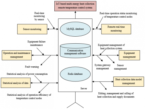
Figure 1. Application architecture of multi-energy heat collection system functions
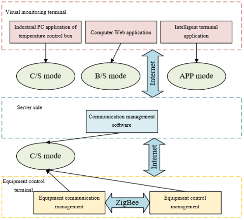
Figure 2. Monitoring mode structure of multi-energy heat collection system
Table 1. Information on the adopted sensors
|
Model |
Purpose |
Range of measurement signal |
Type of output signal |
|
LWGB turbine transmitter |
Measurement of flow |
|
4~20 mA |
|
HTD-SL206 pressure sensor |
Measurement of water pressure |
Choose from -100 KPa~0.6 Mpa ~60 Mpa~120 Mpa |
4-20 mA (two-wire system), 0~5 VDC, 0~10 VDC, 0.5--4.5 VDC (three-wire system) |
|
XFHT-F200-FPB series input static pressure level gauges |
Measurement of water level |
0-0.5M~1M~3M ~5M~10M~20M ~50M~100M~200M (Water level height/depth, with 0.5 m as the minimum range) |
4~20 mA, 0~-10 mA (two-wire system), 0~5 VDC, 0~10 VDC, 0.5~4.5 VDC (three-wire system) |
|
KZW-JPT-A integrated temperature sensor |
Measurement of water temperature |
-200-450℃, accuracy ± 0.2% |
Two-wire system 4~-20 mA |
Figure 1 shows the application architecture of six multi-energy heat collection system functions, namely, remote real-time monitoring, sensor monitoring and management, heat collection supply document management, operation and maintenance management module, equipment management, and data statistics and analysis. Three modes, Browser/Server (B/S), Client/Server (C/S) and APP, were used for the hybrid construction of the remote monitoring architecture of the system. Figure 2 shows the detailed implementation process of the monitoring architecture mode.
The mainly detected data of multi-energy heat collection system included four aspects, namely, water temperature, water level, water pressure and flow. Table 1 shows the information on the adopted sensors, that is, the model, purpose and output signal characteristics of the sensors.
For the IoT-based remote temperature control of multi-energy heat collection, an accurate model is usually required to derive an effective controller. However, due to the inaccurate simulation performance, the traditional model is not suitable for the remote temperature control design. Therefore, this paper developed a multi-energy heat collection system model without losing simulation performance using stochastic modeling ideas.
The heat generated by clean energy was stochastic rather than deterministic, leading to indeterministic data measured by sensors. Stochastic model accurately reflected the temperature changes of the system. At the same time, the stochastic disturbance of objective factors, such as climate and location, might help stabilize the system.
This paper focused on the temperature stochastic modeling and parameter estimation of multi-energy heat collection system. Considering the disturbance of heat, produced by clean energy, by objective factors, such as climate and location, based on the assumption of independent and uniformly distributed disturbance, this paper constructed a stochastic differential equation model of the system, and estimated the drift and diffusion terms using the maximum likelihood estimation method.
Let σwater be the density of tap water, De,water be the specific heat capacity of tap water, U be the volume of tap water participating in heat exchange in the system, Oim be the water inlet temperature of the system, Wcov-water be the heat flux between solar energy heat collection input module and internal tap water in the system, Wflr-water be the heat flux between external air and internal tap water, Wass-water be the heat flux between other clean energy auxiliary heat energy modules and internal tap water, and Wvent be the heat flux loss of tap water caused by objective factors. The following formula gave the duration temperature model expression of the system:
$\begin{aligned} & \frac{\sigma_{\text {water }} D_{e, \text { water }} U d O_{\text {in }}(o)}{d o}= W_{\text {cov_water }}+W_{\text{flr_water}}+W_{\text {ass_water }}+W_{\text {vent }}\end{aligned}$ (1)
Let Xd be the solar panel coverage area of the system, Xh be the heat exchange between solar panel and internal tap water, and Oout be the outlet water temperature of the system. According to the thermodynamic principle, the calculation formula of the heat flux between the solar energy heat collection input module and the internal tap water in the system was:
${{W}_{\operatorname{cov}\_water}}=1.7\frac{{{X}_{d}}}{{{X}_{h}}}{{\left| {{O}_{out}}-{{O}_{in}} \right|}^{0.31}}\left( {{O}_{out}}-{{O}_{in}} \right)$ (2)
Let Oflr be the external air temperature of the system, and lflr-water be the temperature transfer coefficient from external air to tap water in the system. Similarly, the heat flux calculation formula between external air and internal tap water was constructed as follows:
${{W}_{flr\_water}}={{l}_{flr\_water}}{{X}_{h}}\left( {{O}_{flr}}-{{O}_{in}} \right)$ (3)
lflr-water was obtained from the following formula:
${{l}_{flr\_air}}=\left\{ \begin{align} & 1.7{{\left( {{O}_{in}}-{{O}_{flr}} \right)}^{0.33}},{{O}_{flr}}>{{O}_{in}} \\ & 1.3{{\left( {{O}_{in}}-{{O}_{flr}} \right)}^{0.25}},{{O}_{flr}}<{{O}_{in}} \\ \end{align} \right.$ (4)
Let δwater be the heat energy absorption coefficient of tap water, and SEglob be the heat energy supply of other clean energy resources. Then the heat flux between the auxiliary heat energy module of other clean energy resources and the internal tap water was calculated as follows:
${{W}_{ass\_water}}={{\delta }_{water}}\cdot {{X}_{d}}\cdot S{{E}_{glob}}$ (5)
Let Ψvent be the occurrence probability of objective factors, then there was the following formula for calculating the heat flux loss of tap water caused by those factors:
${{W}_{vent}}={{\sigma }_{water}}{{D}_{e,water}}{{\Psi }_{vent}}\left( {{O}_{out}}-{{O}_{in}} \right)$ (6)
It was difficult to calculate Ψvent accurately considering the influence of objective factors, such as season, climate and location. Let αTC and ωTC be the undetermined constants, and the disturbance of objective factors was regarded as the derivative of Brownian motion Y(o), that is, Y(o)=dY(o)/do, then there was:
${{W}_{vent}}={{\sigma }_{water}}{{D}_{e,water}}\alpha _{TC}^{{}}\left( {{O}_{out}}-{{O}_{in}} \right)+{{\omega }_{TC}}Y\left( o \right)$ (7)
The above formula was transformed into the form of nonlinear stochastic differential equation:
$d{{O}_{in}}\left( o \right)=g\left( {{O}_{out}},{{O}_{in}},{{O}_{flr}} \right)do+{{\omega }_{TC}}dY\left( o \right)$ (8)
where,
$\begin{aligned} & g\left(O_{\text {out }}, O_{\text {in }}, O_{f l r}\right)= \frac{1.7 X_d}{\sigma_{\text {air }} D_{e, \text { water }} U X_h}\left|O_{\text {out }}-O_{\text {in }}\right|^{0.31}\left(O_{\text {out }}-O_{\text {in }}\right) +\frac{l_{f l_{\text {water }}} X_g}{\sigma_{\text {water }} D_{e, \text { water }} U}\left(O_{f t t}-O_{\text {in }}\right) +\frac{\delta_{\text {water }} \cdot X_d \cdot S E_{\text {glob }}}{\sigma_{\text {air }} D_{e, \text { water }} U X_h}+\frac{\alpha_{T C}}{U}\left(O_{\text {out }}-O_{\text {in }}\right)\end{aligned}$ (9)
At the same time, when the continuous time path of parameters in the system was observed at equidistant time points, let Δo be the discretization step and ρi be the independent parameter sequence M(0,1), then, there was the following based on formula 8:
$\begin{align} & O_{in}^{i}=O_{in}^{i-k}+g\left( O_{out}^{i-k},O_{in}^{i-k},O_{flr}^{i-k} \right)\Delta o +{{\omega }_{TC}}\sqrt{\Delta o{{\rho }_{i}}},i=1,2,... \\ \end{align}$ (10)
Let O0, O1, O2...Om be the parameter observation sequence based on the above formula, and Gi-1=ε(Oj,j≤i-1), then the conditional probability density function expression of Gi-1,Oi was given by the following formula:
$\begin{aligned} & g\left(O_i / G_{i-1}\right)=\frac{1}{\sqrt{2 \pi \Delta o} \omega_{T C}} \exp \left\{\frac{1}{-2 \omega_{T C \Delta o}^2}\left[O_{\text {in }}^i-O_{\text {out }}^{i-l}-g\left(O_{\text {out }}^{i-l}, O_{i n}^{i-l}, O_{f r i}^{i-1}\right) \Delta o\right]^2\right\}\end{aligned}$ (11)
For the given G0, the following formula gave the joint conditional probability density function expression of (O1, O2...Om):
$\begin{aligned} & \left(O_1, O_2, \ldots, O_m \mid G_0\right)=\left(\frac{1}{\sqrt{2 \pi \Delta o} \omega_{T C}}\right)^n \\ & \coprod_{i=1}^n \exp \left\{\frac{1}{-2 \theta_{T C \Delta o}^2}\left[\begin{array}{l}O_{\text {in }}^i-O_{\text {out }}^{i-l}- \\ g\left(O_{\text {out }}^{i-k}, O_{\text {in }}^{i-1}, O_{f l r}^i\right) \Delta o\end{array}\right]^2\right\}\end{aligned}$ (12)
The log-likelihood function was given by the following formula:
$\begin{aligned} & K_m\left(\alpha_{T C}, \omega_{T C}\right)=-\frac{m}{2} \log 2 \pi \Delta o-m \log \omega_{T C} -\frac{1}{-2 \omega_{T C}^2 \Delta o} \sum_{i=1}^m\left[\begin{array}{l}O_{\text {in }}^i-O_{o u t}^{i-1}- \\ g\left(O_{\text {out }}^{i-1}, O_{\text {in }}^{i-1}, O_{f l r}^i\right) \Delta o\end{array}\right]^2\end{aligned}$ (13)
$\left\{\begin{array}{l}\frac{\partial K_m\left(\alpha_{T C}, \omega_{T C}\right)}{\partial \phi_{T C}}=0 \\ \frac{\partial K_m\left(\alpha_{T C}, \omega_{T C}\right)}{\partial \omega_{T C}}=0\end{array}\right.$ (14)
Based on the above analysis, the following was obtained:
$\left\{\begin{array}{l}\sum_{i=1}^m\left[O_{\text {in }}^i-O_{\text {out }}^{i-1}-g\left(O_{\text {out }}^{i-1}, O_{\text {in }}^{i-1}, O_{f l r}^{i-1}\right) \Delta o\right]=0 \\ -\frac{m}{\omega_{T C}}+\frac{1}{3 \omega_{T C}^3 \Delta o} \sum_{i=1}^m\left[\begin{array}{l}O_{\text {in }}^i-O_{\text {out }}^{i-1}- \\ g\left(O_{\text {out }}^{i-1}, O_{i n}^{i-1}, O_{f l r}^{i-1}\right) \Delta o\end{array}\right]^2=0\end{array}\right.$ (15)
Further, the following was obtained:
$\left\{\begin{array}{l}\hat{\alpha}_{T C}=\frac{\sum_{i=1}^m\left[O_{i n}^i-O_{i n}^{i-1}-Y_{i-1}\right]}{\sum_{i=1}^m\left(O_{\text {out }}^i-O_{i n}^{i-1}\right) \Delta o} \\ \hat{\omega}_{T C}=\sqrt{\frac{\sum_{i=1}^m\left[O_{i n}^i-O_{\text {out }}^{i-1}-g\left(O_{\text {in }}^i, O_{\text {out }}^{i-1}-g\left(O_{o u t}^{i-1}, O_{\text {in }}^{i-1}, O_{\text {flr }}^i\right) \Delta o\right)\right]^2}{3 m \Delta o}}\end{array}\right.$ (16)
where,
$\begin{aligned} & Y_{i-1}=\frac{1.7 X_d}{\sigma_{\text {water }} D_{e, \text { water }} U X_h}\left|O_{o u t}^{i-1}-O_{i m}^{i-1}\right|^{0.31} \left(O_{\text {out }}^{i-1}-O_{i n}^{i-1}\right)+\frac{l_{f l r_{a i r}} X_h}{\sigma_{\text {water }} D_{e, \text { water }} U}\left(O_{f l r}^{i-1}-O_{i n}^{i-1}\right) +\frac{\delta_{\text {water }} \cdot X_d \cdot S E_{\text {glob }}}{\sigma_{\text {water }} D_{e, \text { water }} U X_h}\end{aligned}$ (17)
After controlling the multi-energy heat collection system at time l, the predicted value of the system at the next time might deviate from the actual value, because the actual remote temperature control process was easily affected by objective factors (season, climate, location, etc.) and unknown uncertain factors (model error, time-varying, etc.). In order to correct this situation, it was necessary to fully consider the real-time information of multi-energy heat collection system, and to conduct feedback correction on the remote temperature control system, thus avoiding the occurrence of false remote temperature control system solution values, and at the same time reducing the divergence probability of remote temperature control system. Therefore, this paper chose to make full use of the error information of the process, instead of correcting after all the temperature control increments worked, thus completing the correction of the output predicted value. The following formula gave the expression of the first control action, among the first implemented control increment ΔvN (l) for N time starting from the current time, at time o=lO:
$\begin{aligned} & \Delta v(l)=d^T \Delta v_N(l)= d^T\left(X^T W X+S\right)^{-1} X^T W\left[\theta_e(l)-\tilde{b}_{E 0}(l)\right] =c^T\left[\theta_e(l)-\tilde{b}_{E 0}(l)\right]\end{aligned}$ (18)
$v\left( l \right)=v\left( l-1 \right)+\Delta v\left( l \right)$ (19)
${{c}^{T}}={{D}^{T}}{{\left( {{X}^{T}}W+X \right)}^{-1}}{{S}^{T}}X={{W}_{1}}\left( {{c}_{2}}\cdot {{c}_{E}} \right)$ (20)
Let ΔvN(l) be the optimal solution at the time of o=(l+1)O, ∆v(l+1) be the second component, b(l+1) be the actual output of the multi-energy heat collection system object, and ḃ1(l+k|l) be the prediction output of the model, which is the first component of ḃM1(l). The output prediction of the system in the future was mainly affected by the control increment ∆v(l), because Δv(l) was already applied to the system object. Therefore, b(l+1) should be detected and compared with ḃ1(l+k|l), instead of continuing to implement ∆v(l+1), thus forming the output error.
$p\left( l+1 \right)=b\left( l+1 \right)-{{\dot{b}}_{1}}\left( l+1|l \right)$ (21)
The output error information reflected the influence of objective factors and unknown uncertain factors (model mismatch, time-varying, etc.) on the system output. Considering the existence of prediction error, the output value prediction of the remote temperature control system at all time also needed to be corrected. This paper predicted the future output error using the time series method. Let p(l+1) be the real-time error of the remote temperature control system, and ḃCE(l+1) be the output of the predicted system at time o=(l+i)O(i=1,...,M) after error correction at time o=(l+1)O, then ḃCE(l+1) was obtained by weighting the coefficient fi(i-1,2,... ,M) on p(l+1):
${{\dot{b}}_{CE}}\left( l+1 \right)={{\dot{b}}_{N1}}\left( l \right)+fp\left( l+1 \right)$ (22)
$\dot{b}_{C E}(l+1)=\left[\begin{array}{l}\dot{b}_{C E}(l+1 \mid l+1) \\ \vdots \\ \dot{b}_{C E}(l+M \mid l+1)\end{array}\right]$ (23)
where, the error correction vector f was:
$f=\left[\begin{array}{l}f_1 \\ \vdots \\ f_M\end{array}\right]$ (24)
According to the above derivation, after being corrected, except the first item, other items in ḃCE(l+1) are the predicted values of system output of time o=(l+2)O without the influence of Δv(l+1) at time o=(l+1)O. Those items were regarded as the first M-1 components of ḃM0(l+1) at time o=(l+1)O, that is:
$\begin{aligned} & \dot{b}_0(l+1+i \mid l+1)=\dot{b}_{C E}(l+1+i \mid l+1), i=1, \ldots, M-1\end{aligned}$ (25)
The prediction of the output of i=(l+1+M)O at time o=(l+1)O was the last component of ḃM0(l+1). Due to the influence of model truncation, the prediction was approximated by ḃ0(l+1|l+1). That is, ḃM0(l+M|l+1) was expressed using the vector form in the following formula:
$\dot{b}_{M 0}(l+1)=R \cdot \dot{b}_{C E}(l+1)$ (26)
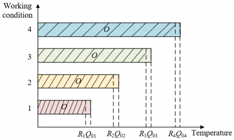
ḃM0(l+1) was obtained at time o=(l+1)O, which pushed ahead the control process of remote temperature control system, thus optimizing the temperature control strategy at time l+1. The whole control continued to move forward, jointly affected by the model optimization of multi-energy heat collection system and feedback correction. Figure 3 shows the proportional control diagram of temperature control time in different working conditions.
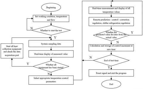
According to the above analysis, the remote temperature control strategy proposed in this paper was divided into three parts: prediction, control and correction. Based on Δv(l) of each sampling time, the control quantity v(l) was calculated through digital integration operation and applied to the system object, and ḃM1(l) was also calculated through multiplication operation with step response vector. At the next sampling time, b(l+k) was first detected and the output error p(l+1) was calculated. As the control process progressed, the corrected ḃCE(l+1) shifted to generate a new initial prediction value ḃM0(l+1). The new time was redefined as l time by the time-displacement operator. The calculation of the control increment at the new time was completed based on the expected system output and the components of the initial predicted value ḃM0(l). The remote temperature control process of multi-energy heat collection was repeated online through this cycle. Figure 4 shows the flow chart of the main program.
Figure 3. Schematic diagram of proportional control of temperature control time in different working conditions
Figure 4. Flow chart of temperature control main program
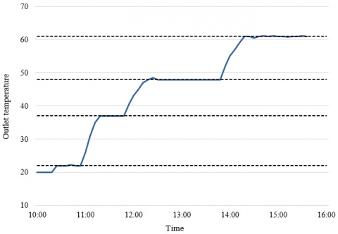
Figure 5. Water tank outlet temperature curve in all working conditions
According to the remote temperature control mode of multi-energy heat collection proposed in this paper, Figure 5 shows the outlet temperature change curve of water tank in all working conditions of the system. According to the experiment, with the influence of objective factors (season, climate and location, etc.) and unknown uncertain factors (model error, time-varying, etc.), the system control kept the outlet temperature of water tank constant in each working condition, and the temperature fluctuation was controlled within the preset range.
According to the disturbance degree of objective and uncertain factors and without considering the interactions of those factors, this paper selected the calculation orthogonal table of control increment at the new time to determine the experimental scheme. Table 2 shows the proportional, integral and derivative (PID) parameters of the thyristor controlling the system heat flow and the mean square error of inlet temperature of the heat collection tank in all schemes.
Table 2. Experimental results of remote temperature control strategy of multi-energy heat collection
|
Factors Test No. |
Maximum voltage (V) |
P |
1 |
D |
Inlet temperature variance |
|
1 |
2 |
3 |
4 |
||
|
1 |
1(2.5) |
1(50) |
1(3) |
1(1) |
0.01097 |
|
2 |
1(2.5) |
2(55) |
2(3.5) |
2(1.5) |
0.243753 |
|
3 |
1(2.5) |
3(60) |
3(4) |
2(1.5) |
0.11257 |
|
4 |
2(2.6) |
1(50) |
1(3) |
3(2) |
0.025006 |
|
5 |
2(2.6) |
2(55) |
2(3.5) |
1(1) |
0.017863 |
|
6 |
2(2.6) |
3(60) |
3(4) |
1(1) |
0.064259 |
|
7 |
3(2.7) |
1(50) |
1(3) |
2(1.5) |
0.029923 |
|
8 |
3(2.7) |
2(55) |
2(3.5) |
2(1.5) |
0.03794 |
|
9 |
3(2.7) |
3(60) |
3(4) |
3(2) |
0.26751 |
|
10 |
4(2.8) |
1(50) |
1(3) |
1(1) |
0.03672 |
|
11 |
4(2.8) |
2(55) |
2(3.5) |
1(1) |
0.029754 |
|
12 |
4(2.8) |
3(60) |
3(4) |
2(1.5) |
0.039252 |
|
13 |
5(2.9) |
1(50) |
1(3) |
2(1.5) |
0.036411 |
|
14 |
5(2.9) |
2(55) |
2(3.5) |
3(2) |
0.034829 |
|
15 |
5(2.9) |
3(60) |
3(4) |
1(1) |
0.035366 |
|
16 |
6(3.0) |
1(50) |
1(3) |
2(1.5) |
0.037524 |
|
17 |
6(3.0) |
2(55) |
2(3.5) |
3(2) |
0.041916 |
|
18 |
6(3.0) |
3(60) |
3(4) |
1(1) |
0.036136 |
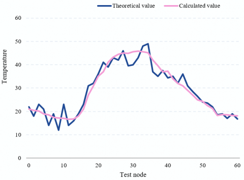
1) Test node temperature
2) Temperature error
Figure 6. Model test results
Table 3. Variance analysis of multi-energy heat collection remote temperature control experiment
|
Level |
Maximum voltage |
P |
I |
D |
|
1 |
0.12236 |
0.02976 |
0.02954 |
0.03517 |
|
2 |
0.03521 |
0.06754 |
0.06751 |
0.0619 |
|
3 |
0.03157 |
0.0568 |
0.0536 |
0.04571 |
|
4 |
0.0634 |
|
|
|
|
5 |
0.03576 |
|
|
|
|
6 |
0.03815 |
|
|
|
|
Delta |
0.0906 |
0.03712 |
0.03851 |
0.03526 |
|
Rank |
1 |
3 |
2 |
4 |
Figure 6 shows the model test results, that is, the error values of measured and predicted temperature and theoretical temperature at different test nodes. The actual measured and predicted temperature of the test node was closely related to the solar radiation value, because the solar energy collection module in the multi-energy heat collection system was the core heating module, and other clean energy modules were the auxiliary thermal energy modules. The figure shows that the temperature of the system in this experiment changes with time, which verified the effectiveness of the model in this paper in the remote temperature control results of the system.
The data of 18 groups of experimental results were further analyzed. Table 3 shows the variance analysis results of the remote temperature control experiment.
According to the table, when the thermal flow of the system was controlled by the thyristor, the analog input was the main factor of remote temperature control of multi-energy heat collection, and the PID control parameters were the secondary factor of temperature control. Based on the variance analysis results, the optimal multi-energy heat collection cooperation strategy was obtained. That is, the analog input maximum voltage of thyristor was 2.6 V, and the PID control parameters were 51, 4, and 2.
According to the analysis results, when the heat produced by clean energy was disturbed by objective factors, such as climate and location, the controlled multi-energy heat collection system had rapid temperature response, short adjustment time, and relatively ideal control effect and robust performance.
This paper studied the IoT-based remote temperature control strategy of multi-energy heat collection. First, this paper gave the application architecture of multi-energy heat collection system functions, and developed a system model without losing simulation performance using stochastic modeling ideas. Second, the paper selected to make full use of the error information of the process, thus correcting the predicted value of remote temperature control output. According to the remote temperature control mode of multi-energy heat collection proposed in this paper, this paper drew the outlet temperature change curve of water tank in all working conditions of the system. In addition, this paper collected the PID parameters of the thyristor controlling the system heat flow and the mean square error of inlet temperature of heat collection water tank in different experimental schemes. This paper gave the error values of measured and predicted temperature and theoretical temperature at different test nodes, which verified that the model in this paper obtained effective results in controlling the remote temperature of multi-energy heat collection system. Then this paper further analyzed the variance of remote temperature control experiment of multi-energy heat collection. The experimental results showed that the controlled multi-energy heat collection system had rapid temperature response, short adjustment time, and relatively ideal control effect and robust performance.
[1] Rosselló, J.M., Ohl, C.D. (2023). Clean production and characterization of nanobubbles using laser energy deposition. Ultrasonics Sonochemistry, 94: 106321. https://doi.org/10.1016/j.ultsonch.2023.106321
[2] Valayer, P.J., Vidal, O., Wouters, N., van Loosdrecht, M.C. (2019). The full energy cost of avoiding CO2: A clean-energy booking provision for a vigorous energy transition. Journal of Cleaner Production, 237: 117820. https://doi.org/10.1016/j.jclepro.2019.117820
[3] Shukla, U., Bajpai, R. (2019). Nuclear power plants in India: achieving clean and green energy. International Journal of Nuclear Energy Science and Technology, 13(1): 87-97. https://doi.org/10.1504/IJNEST.2019.10020882
[4] Galante, R.M., Vargas, J.V., Balmant, W., Ordonez, J.C., Mariano, A.B. (2019). Clean energy from municipal solid waste (MSW). In Energy Sustainability. American Society of Mechanical Engineers, 59094: V001T16A004. https://doi.org/10.1115/ES2019-3961
[5] Newell, R.G., Pizer, W.A., Raimi, D. (2019). US federal government subsidies for clean energy: Design choices and implications. Energy Economics, 80: 831-841. https://doi.org/10.1016/j.eneco.2019.02.018
[6] Wu, Z.S., Li, X., Wang, F., Bao, X. (2019). DICP's 70th anniversary special issue on advanced materials for clean energy. Advanced Materials, 31(50): 1905710. https://doi.org/10.1002/adma.201905710
[7] Wang, H., Bi, X., Clift, R. (2023). Clean energy strategies and pathways to meet British Columbia's decarbonization targets. The Canadian Journal of Chemical Engineering, 101(1): 81-96. https://doi.org/10.1002/cjce.24654
[8] Bei, J., Wang, C. (2023). Renewable energy resources and sustainable development goals: Evidence based on green finance, clean energy and environmentally friendly investment. Resources Policy, 80: 103194. https://doi.org/10.1016/j.resourpol.2022.103194
[9] Martinez-Sierra, D., García-Samper, M., Hernández-Palma, H., Niebles-Nuñez, W. (2019). Energy management in the health sector of Colombia: a case of clean and sustainable development. Información Tecnológica, 30(5): 47-56. https://doi.org/10.4067/S0718-07642019000500047
[10] Dahbi, S., Aziz, A., Messaoudi, A., Mazozi, I., Kassmi, K., Benazzi, N. (2018). Management of excess energy in a photovoltaic/grid system by production of clean hydrogen. International Journal of Hydrogen Energy, 43(10): 5283-5299. https://doi.org/10.1016/j.ijhydene.2017.11.022
[11] Aghdam, F.H., Ghaemi, S., Kalantari, N.T. (2018). Evaluation of loss minimization on the energy management of multi-microgrid based smart distribution network in the presence of emission constraints and clean productions. Journal of Cleaner Production, 196: 185-201. https://doi.org/10.1016/j.jclepro.2018.06.023
[12] Wang, W., Wang, D., Jia, H., He, G., Hu, Q.E., Sui, P.C., Fan, M. (2017). Performance evaluation of a hydrogen-based clean energy hub with electrolyzers as a self-regulating demand response management mechanism. Energies, 10(8): 1211. https://doi.org/10.3390/en10081211
[13] Sharma, R. (2016). Management of clean coal technologies and biofuels for cleaner energy policy and planning. Energy Sources, Part B: Economics, Planning, and Policy, 11(7): 597-607. https://doi.org/10.1080/15567249.2012.715722
[14] Yuksel, I. (2015). Water management for sustainable and clean energy in Turkey. Energy Reports, 1: 129-133. https://doi.org/10.1016/j.egyr.2015.05.001
[15] Weng, C., Feng, X., Sun, J., Ouyang, M., Peng, H. (2015). Battery SOH management research in the US-China clean energy research center-clean vehicle consortium. IFAC-PapersOnLine, 48(15): 448-453. https://doi.org/10.1016/j.ifacol.2015.10.064
[16] Liu, J., Cao, X., Xu, Z., Guan, X., Dong, X., Wang, C. (2021). Resilient operation of multi-energy industrial park based on integrated hydrogen-electricity-heat microgrids. International Journal of Hydrogen Energy, 46(57): 28855-28869. https://doi.org/10.1016/j.ijhydene.2020.11.229
[17] Meng, Z., Wang, S., Zhao, Q., Zheng, Z., Feng, L. (2021). Reliability evaluation of electricity-gas-heat multi-energy consumption based on user experience. International Journal of Electrical Power & Energy Systems, 130: 106926. https://doi.org/10.1016/j.ijepes.2021.106926
[18] Hou, H., Liu, P., Xiao, Z., Deng, X., Huang, L., Zhang, R., Xie, C. (2021). Capacity configuration optimization of standalone multi‐energy hub considering electricity, heat and hydrogen uncertainty. Energy Conversion and Economics, 2(3): 122-132. https://doi.org/10.1049/enc2.12028
[19] Diao, H., Li, P. (2021). Robust coordinated operation of an integrated electricity-heat system with multi-energy microgrids considering uncertain interactive power. In 2021 IEEE 5th Conference on Energy Internet and Energy System Integration (EI2), IEEE, pp. 184-189. https://doi.org/10.1109/EI252483.2021.9713139
[20] Park, C., Jung, Y., Lim, K., Kim, B., Kang, Y., Ju, H. (2021). Analysis of a phosphoric acid fuel cell-based multi-energy hub system for heat, power, and hydrogen generation. Applied Thermal Engineering, 189: 116715. https://doi.org/10.1016/j.applthermaleng.2021.116715
[21] Singh, A., Sharma, S., Verma, A. (2020). Coordination framework for optimal multi-energy dispatch in heat and power distribution networks. In 2020 IEEE International Conference on Power Electronics, Drives and Energy Systems (PEDES), IEEE, pp. 1-5. https://doi.org/10.1109/PEDES49360.2020.9379854
[22] Hu, Z., He, C. (2022). Economic dispatch of park-level multi-energy systems considering the uncertainty of wind and solar with gas-heat energy storages. In 2022 4th International Conference on Power and Energy Technology (ICPET), IEEE, pp. 834-840. https://doi.org/10.1109/ICPET55165.2022.9918231
[23] van der Roest, E., Beernink, S., Hartog, N., van der Hoek, J.P., Bloemendal, M. (2021). Towards sustainable heat supply with decentralized multi-energy systems by integration of subsurface seasonal heat storage. Energies, 14(23): 7958. https://doi.org/10.3390/en14237958
[24] Fu, J., Yang, D., Sun, Y., Zhang, H., Li, B., Zhang, X. (2020). Research on optimal dispatching of multi-energy flow system considering heat network loss under different optimization objectives. In 2020 10th International Conference on Power and Energy Systems (ICPES), IEEE, pp. 493-498. https://doi.org/10.1109/ICPES51309.2020.9349685
[25] He, S., Liu, N., Li, R. (2020). Multi-objective coordinated operation for multi-energy hub considering heat network model. In 2020 IEEE 3rd Student Conference on Electrical Machines and Systems (SCEMS), IEEE, pp. 830-836. https://doi.org/10.1109/SCEMS48876.2020.9352262
[26] Yang, D., Fu, J., Sun, Y., Zhang, H., Li, B., Zhang, X. (2020). Research on nodal energy price of multi-energy flow system considering heat network loss. In 2020 IEEE 4th Conference on Energy Internet and Energy System Integration (EI2), IEEE, pp. 2523-2527. https://doi.org/10.1109/EI250167.2020.9347331