Gugliemina Mutani* | Simone Beltramino
(This article is part of the Special Issue 7th int. Conf. AIGE-IIETA and 16th Conf. AIGE)
© 2022 IIETA. This article is published by IIETA and is licensed under the CC BY 4.0 license (http://creativecommons.org/licenses/by/4.0/).
OPEN ACCESS
Climate changes and urban population growth are increasing the heat island effects in cities, making the urban outdoor environment less comfortable for people. Consequently, improving the thermal comfort conditions of urban open spaces could be considered one important challenge that cities can pursue in the upcoming years. As a first step, this work aims to assess which GIS tools are most useful for evaluating place-based outdoor thermal comfort conditions at urban scale. The UMEP-SOLWEIG (QGIS) tool was described and compared with ENVI-met, to calculate the thermal comfort indexes in different outdoor spaces, during extreme summer and winter conditions, in the city of Turin. These tools can be easily implemented in platforms to represent the spatial distribution of thermal comfort conditions in cities for prioritizing strategies and defining effective actions within land-use plans. This type of representation is crucial as it provides very comprehensible results to urban or regional planners and policy-makers. In this study, UMEP-SOLWEIG appeared to be the most suitable tool since it is the best compromise between simulation time and accuracy at urban scale.
outdoor thermal comfort, UMEP-SOLWEIG, ENVI-met, sky view factor, mean radiant temperature, urban surfaces, urban morphology, urban scale
Climate changes and urban population growth are increasing the heat island effects in cities, causing environmental impacts and making the urban outdoor environment less comfortable for people. Urban space is a limited and precious resource that must be exploited to the fullest [1]. Therefore, improving the thermal comfort conditions of urban outdoor spaces could be considered one important challenge for cities, also considering how people use more outdoor spaces after the COVID-19 pandemic. This work contributes to defining which urban characteristics support sustainability, depending on urban context and climate conditions. Many studies have focused on defining metrics to identify and evaluate the most sustainable urban forms [2]. Studies on this topic focus primarily on the relationship between urban density and compactness with sustainability [2, 3]. Some of these studies identify, through correlations, compact cities as more energy-sustainable reducing energy consumption in cities, while others show their relatively potential to use renewable energy sources. Currently, there is a lack of guidelines related to urban density indicators and their relationship to outdoor thermal comfort. Recently, several studies have focused on methods to optimize outdoor thermal comfort in cities. Nevertheless, a gap remains between scientific best practices and their implementations considering the real urban context. Numerical models and tools are essential for the analysis of outdoor thermal comfort as they take into account both urban forms and climates through predictive models. Thanks to numerical models it is possible to analyze and compare different urban design scenarios, allowing the simulation under different meteorological and boundary conditions [4].
The aim of this work is to present the current software to evaluate local climate and thermal comfort conditions in cities, helping to define the most appropriate type of tool for urban or territorial scale. This work evaluates the outdoor thermal comfort conditions with local scale and urban scale tools in the city of Turin. The evaluation has been done in the hotter summer day and the coldest winter day during 2015 to consider two opposite climatic conditions of thermal stress. The results of this work provide urban thermal comfort maps and graphs to support urban planners, useful to implement guidelines for checking and improving the livability of outdoor spaces.
A remarkable amount of research papers have analyzed the outdoor thermal comfort conditions in urban environments, and some of them have been published recently [4]. In particular, the tools used to evaluate thermal comfort conditions can be classified based on their spatial scale in [5]:
Local scale tools: they use very accurate, complex, and time-consuming models, are useful for advanced feasibility studies, and for the design phase of blocks of buildings and little neighborhoods. Most of the research papers on these tools have focused on the evaluation of outdoor thermal comfort at the local scale using finite element calculation models. The high level of resolution allows the study of local scale interactions between humans, buildings, surfaces, and plants. One of the most used tools is ENVI-met [6];
Urban scale tools: are less common in literature and most of them are based on Geographic Information System (GIS) or the open-source Quantum GIS (QGIS) software. They are based on more simplified models for the calculation of thermal comfort variables, returning lower accuracy results, but the possibility to consider a larger urban area with lower simulation times. A good level of resolution of the urban context allows to study the interactions between the urban environment and outdoor thermal comfort conditions. One of the most used tools is UMEP within SOLWEIG QGIS tool [7].
The articles that consider the QGIS with UMEP-SOLWEIG tool are few especially considering different climate conditions, various contexts, and scales [4]. Specifically, this tool has been applied in Gothenburg [8], a continental climate, to assess how urban form can influence outdoor thermal comfort conditions; in Hong Kong [9], a subtropical climate, to analyze how the mean radiant temperature (Tmrt) changes in high-density urban contexts. In addition, UMEP-SOLWEIG was used to evaluate the influence on Tmrt and thermal comfort conditions of the land cover [10] and with various shares of vegetation [11-13].
This work evaluates thermal comfort conditions at a block of buildings-district-urban scale utilizing UMEP-SOLWEIG considering different built contexts in the city of Turin, in Italy. Then, a comparison between UMEP-SOLWEIG and ENVI-met is reported considering a summer day and a winter day.
The following section presents the thermal comfort assessment at urban scale highlighting the main differences between UMEP-SOLWEIG and ENVI-met in terms of input data, output data, accuracy, and simulation times for various case-studies. In particular, the models analyzed are ENVI-met 5.0.2 and UMEP-SOLWEIG v2021a.
2.1 ENVI-met 5.0.2
ENVI-met was analyzed, as it is the most widely used Computational Fluid Dynamics (CFD) tool in literature for local climate and thermal comfort analyses [6]. ENVI-met is a holistic tool (considering the effect of the atmosphere, soil, vegetation, and built environment), based on finite elements numerical approach that is used for the calculation of outdoor thermal comfort. It is designed for local scale analyses with a grid resolution of 0.5-10 m considering a time period of 24-48 hours and a time step of 1 second to 1 hour. ENVI-met simulates radiation fluxes, temperatures, wind flows, air humidities, and Tmrt for each time and spatial step. The spatial resolution is limited to 250×250×25 grids, due to its complexity. Table 1 reports the main characteristics of ENVI-met describing the input and output data with the more typical applications.
2.2 UMEP and SOLWEIG v2021a
The selection of a QGIS tool for urban applications is based on the availability of a limited number of input parameters for the whole urban environment and considering that the simulation time must be reasonable, if the objective is to compare design alternatives in districts. In this work, the Urban Multi-scale Environmental Predictor (UMEP) was used to evaluate the outdoor thermal comfort conditions in a city; UMEP is an open-source tool of QGIS to access climate-sensitive urban planning. For the analysis of outdoor thermal comfort, the SOlar and LongWave Environmental Irradiance Geometry model (SOLWEIG) is necessary [7, 14]. SOLWEIG simulates the effects of radiant flux densities and mean radiant temperature (Tmrt) using high-quality Digital Surface Models (DSM), with a maximum of 4 million pixels, and the weather data. In Table 2, it is possible to observe the main differences between this tool and ENVI-met. With UMEP and SOLWEING is possible to calculate the spatial distribution of: wind, air temperatures, outdoor thermal comfort conditions, and climate changes scenarios [14]. Tools and plugins of QGIS are written in Python for free platforms and open-source applications, enabling users to interact with its spatial information. Moreover, with the last version of SOLWEIG [15] is possible to consider 3D vegetation and outdoor surface differences.
Table 1. ENVI-met input and output data
|
Input data |
Output data |
||||
|
Model |
Supported data |
Climatic data |
Simulated variables |
Comfort indexes |
Application |
|
Grid-based model, limited to 250×250×25 grids |
File formats: .INX, .simx, Net-CDF. |
Hourly values of air temperature and relative humidity. Daily data of wind speed and direction (average values) |
Ta, Ts, Q, Tmrt, Ws, Wd*, CO2, and pollutants’ concentration |
PMV, UTCI, PET, SET |
Local scale: building and block of buildings |
*Ta: air temperature; Ts: surface temperature; Q: long-wave and short-wave solar radiation; Tmrt: mean radiant temperature; Ws: wind speed; Wd: wind direction.
Table 2. UMEP-SOLWEIG input and output data
|
Input data |
Output data |
|||||
|
Model |
Supported data |
Climatic data |
Sky View Factor |
Variables |
Comfort indexes |
Application |
|
Digital Elevation Models, maximum 4,000,000 pixels |
Geospatial data: shapefile and raster data type, and text-dbx |
Hourly values of radiation, temperature, air relative humidity, pressure, wind, and rainfall |
For each point of the DEM (considering building, ground, and vegetation) |
Q, Tmrt* |
PET and UTCI only in Points of Interest (POIs) |
Block of building, neighborhood, district and urban scale |
*Q: long-wave and short-wave solar radiation; Tmrt: mean radiant temperature.
Table 2 shows that the data required by QGIS tools are few and simple and the use of SOLWEIG allows identifying all variables for the calculation of thermal comfort indexes, such as solar radiation (Q) and Tmrt. The simulations are processed quickly and most part of the simulation time is taken for the calculation of radiation fluxes and mean radiant temperatures. In addition, this software only allows the calculation of comfort indices (limited to PET and UTCI) at some specified points.
2.2.1 Radiation model
The radiation assessment uses the six-directions approach [16] which calculates shortwave and longwave radiation fluxes arriving from the four cardinal directions, below, and above. SOLWEIG refers to [7, 10, 17] for the short-wave and long-wave radiation fluxes. The horizontal direct (Kdir,horS) and diffuse solar irradiance (KdifS) are calculated according to Eq. (1) and Eq. (2):
$K_{\text {difS }}=S V F \cdot K_{\text {dif }}$ (1)
$K_{\text {dir,horS }}=S L \cdot K_{\text {dir,beam }} \cdot \sin (\beta)$ (2)
where: SVF is the sky view factor; Kdif is the diffuse irradiance from the sky and Kdir,beam is the direct solar irradiance [18] [Wm-2]; SL is the percentage of sunlight area (1 sunny; 0 shadow) and β is the sun’s height angle.
The calculation of radiative fluxes yields the following approximations [18]:
1. The reflected shortwave radiation is equally distributed among the cardinal directions as a function of sun’s height angle and SVF for each point [7, 10];
2. The outdoor surfaces’ temperature is equal to air temperature in the absence of direct solar radiation and after two hours of shadow;
3. For different surface materials, the surface temperature is derived from experimental campaigns;
4. An average surface temperature of soils and walls is used to calculate the components of the solid surface emitted longwave flux when estimating downwelling fluxes.
To evaluate the mean radiant temperature Tmrt, the average radiant flux intensity (R) is defined as the sum of shortwave (Ki) and longwave (Li) radiation (considering the 3D space: i=1-6) according to Eq. (3):
$R=\alpha_k \cdot \sum_{i=1}^6 K_i \cdot F_i+\varepsilon_p \cdot \sum_{i=1}^6 L_i \cdot F_i$ (3)
where: Fi is the form factor between a person and the surrounding surfaces (for a standing person: Fi= 0.06 from above-below and Fi = 0.22 for the four cardinal directions); for a human body, the emissivity is ɛp = 0.97, and the absorption coefficient for shortwave radiation is αk = 0.7 [7].
2.2.2 Net radiation through vegetation
To consider the irradiance that crosses and exceeds vegetation and trees and to consider the seasonal entity of the leaves of deciduous trees, different parameters were used. Typical parameters founded in the literature were used to define the values of Leaf Area Index (LAI) for deciduous trees, defined by Eq. (4a), usually: 5.0 in summer and 0.6 in winter [19-21]. The shortwave transmittance τs, considering diffuse shortwave radiation through leaves, was described by the exponential law Eq. (4b) [19, 20]:
$L A I=\frac{\text { Leaf surface }}{\text { Ground area }}$ (4a)
$\tau_S=e^{-k_S L A I}$ (4b)
where: ks is the coefficient of extinction; considering a spherical tree’s shape: ks= 0.747; the Leaf Area Density LAD can be used too, by dividing the LAI for the height of vegetation.
2.3 Comparison between ENVI-met and UMEP-SOLWEIG software
In literature, some studies have compared UMEP-SOLWEIG with ENVI-met to validate the QGIS tool at the urban scale. In 2015, Jänicke et al. [21] compared the results of SOLWEIG models with three observations in Berlin with good accuracy for the Tmrt but with an overestimation of the radiation amplitude upwards. In 2020, Gála and Kántor [18] compared SOLWEIG with observations with a good agreement, while Hu et al. [22] found lower errors with ENVI-met. In this work, ENVI-met was compared with UMEP-SOLWEIG to validate this last tool under extreme summer and winter weather conditions in a temperate climate, analyzing thermal comfort conditions and some variables used for the calculations (in Table 3).
Table 3. Comparison between ENVI-met and UMEP-SOWEIG tools
|
Models |
Wind |
Ta and RH |
Radiative fluxes |
Pollutant |
Soil |
Vegetation |
Built environment |
|
ENVI-met |
Reynolds-averaged non-hydrostatic Navier-Stokes equations |
Determined by the different sources and sinks of sensible heat and vapor in the model |
Radiation fluxes (avg) consider shading, reflections, building materials, the effect of vegetation |
Pollutant dispersion model is developed by ENVI-met |
The heat conductivity considers the soil water content (Darcy's law). A 3D root model calculates water extraction from the soil |
All plants are treated solving the energy balance of the leaf surface |
Complex buildings can be constructed with no limitations, represented by a thermodynamical model of 7 prognostic calculation nodes |
|
UMEP-SOLWEIG |
Hourly weather data |
Hourly weather data |
Diffuse and direct solar radiation calculation from the global radiation using the approach |
Not calculated |
Grass and natural surfaces have been parameterized considering the DSM [10] |
Tveg is equal to Ta; shortwave and longwave fluxes |
Derived from DSM of buildings and ground |
From Table 3, it can be observed that both tools provide simplifications depending on the objective of their analysis. ENVI-met is complex, time-consuming, and limited in size. It is useful for high spatial and temporal resolution feasibility studies or for the design phase of little neighborhoods. While UMEP-SOLWEIG requires fewer input data, short simulation times and is more suitable for analyses at urban scale. UMEP-SOLWEIG applies substantial simplifications for the atmospheric, soil, vegetation, and built environment models; in particular, by forcing the input meteorological data (Ta, RH, Ws, Wd, I), without modeling them for each grid and time step, like ENVI-met. Lastly, the calculation of thermal comfort indexes is similarly implemented: the Physiological Equivalent Temperature PET is calculated by the Munich Energy Balance Model for Individuals (MEMI); the Universal Thermal Climate Index UTCI is calculated by the same 6th order polynomial regression function.
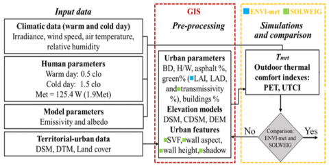
The outdoor thermal comfort in the northern Italian city of Turin was investigated in districts with different built environment characteristics. Following the literature review, ENVI-met is the most widespread software for thermal comfort analyses at the local scale [23, 24], while UMEP-SOLWEIG is the most suitable QGIS tool for urban scale analyses. Therefore, UMEP-SOLWEIG was compared with ENVI-met and then utilized to evaluate local climate and outdoor thermal comfort conditions in two neighborhoods of Turin. Each element of the city was described with 5x5 meters cells. With ENVI-met, this resolution is quite accurate to describe the built environment and outdoor spaces without increasing too much simulation times. The simulations were done considering two critical days: the hottest and the coldest day in the year 2015. The aim was to describe the actual scenario (business-as-usual SBAU) under two different climatic conditions to assess the accuracy of SOLWEIG in calculating outdoor thermal comfort conditions. The results of this analysis allow to evaluate the liveability in different zones and how thermal comfort depends on the characteristics of the urban environments. Figure 1 shows the methodology used in this work: from the identification of input data, the pre-processing phase with the calculation of the variables, and then the simulation of outdoor indexes at urban scale. Finally, for two different neighborhoods, the accuracy of the QGIS tool SOLWEIG was checked in some points by the use of ENVI-met.
3.1 Case study
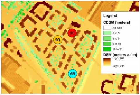
A first analysis at urban scale was implemented on the central District 1 of the city of Turin, to observe the potential of SOLWEIG. Then, two neighborhoods with different characteristics were selected to evaluate the accuracy of this analysis with UPEP-SOLWEIG. The neighborhoods Arquata e Mediterraneo (in Figure 2) were selected because they have similar typologies of land use but different built morphologies (respectively: aspect ratio H/W: 0.27-0.62; buildings’ density: 3.56-6.96 m3/m2 [24]). Then, the results of the simulations with SOLWEIG were compared with ENVI-met considering a warm and a cold day in some points of interest. In Table 4 are reported the main input data of this analysis: emissivity, albedo, and seasonal leaf trend parameters.
Figure 1. Methodology assessment
3.1.1 Territorial-urban data
The main required inputs are elevation data that identify the buildings and infrastructures on the territory, attributing to each cell the height value above sea level (usually in a raster format like images). In particular, the input data that describe the morphology and land-use are the surface model of:
- territory and building altitude with Digital Surface Model (DSM);
- territory with Digital Elevation Model or Digital Terrain Model (respectively DEM and DTM);
- 3D vegetation with Digital Canopy Surface Model (CDSM); trunk heights with Digital Trunk Zone Surface Model (TDSM); TDSM is rarely available but can be estimated with 25% of CDSM [15].
Lastly, the land cover use (identified with numbers from 1 to 7) was uploaded by the technical map of the city [10] to consider the presence of built area but also grass, concrete, and asphalt surfaces.
3.1.2 Weather data
The hourly weather data were acquired from a local weather station. This work compares the warmest and coldest days recorded in 2015, respectively:
- August 7th with an average air temperature of 31.4℃.
- January 1st with an average air temperature of 2.1℃.
The wind speed is quite low during all the seasons (i.e., 0.5-2.3 m/s) because Turin is surrounded by the Alps.
3.1.3 Human parameters
Thermal comfort simulations were implemented considering a 35-year-old male weighing 75 kg and 1.75 meters tall. Thermal comfort conditions were calculated at a height of 1.1 m, considering:
- clothing insulation: 0.5 clo (summer clothing), and 1.5 clo (outdoor winter clothing);
- metabolic rate of a walking man at 2 km/h with 1.9 met or 110 W/m2.
Table 4. Simulations input data
|
Emissivity |
Albedo |
Deciduous trees seasonal leaf trend parameters |
|
Asphalt 0.9; concrete pavement 0.9; walls and roofs 0.9; grass: 0.95. |
Asphalt 0.2; concrete pavement 0.4; walls 0.6; roofs 0.4; grass 0.2. |
ENVI-met: spherical shape, height of 5-15 m: LAI=5.0 in summer; LAI=0.6 in winter. SOLWEIG: from a 3D model “CDSM”, $\tau_s$= 2% in summer and $\tau_s$= 64% in winter. |
(a) Mediterraneo district
(b) Arquata district
Figure 2. Digital Surface Model DSM and points analized: UC = urban courtyard, SQ = square, GR = green area
3.1.4 Pre-processing
The Sky View Factor was calculated by considering vegetation and buildings with the DSM and CDSM [15] (in Figures 2a and 2b). CDSM, DSM, and DEM were extracted from the Lidar dataset with a resolution of 5m x 5m. Then, the height of the walls and their orientation were calculated with Wall-height and Aspect tools provided by UMEP.
The transmissivity of trees τs was considered constant and equal to 2% in summer and 64% in winter [17]. Values of the coefficient of extinction ks considers the trees’ shape [20, 22, 25].
In Figure 3, some steps of the simulation with SOLWEING on the central District 1 of Turin (i.e., 688 ha) on August 7th, 2015 at 1 pm are shown. Simulation times are mainly related to the collecting of input data (which lasted 3 hours), the simulation of sky view factor SVF, and the Tmrt calculations (respectively 10 and 2 hours). Then the outdoor thermal comfort was calculated in three points of interest for the two critical days with hourly time steps. The simulation times were overall between 16 and 17 hours. In Figure 3a the SVF is represented by describing the urban morphology. Then in Figure 3b, the Tmrt was calculated knowing the geometries and surfaces’ materials of the built environment respecting the human body for each point of the grid (5m x 5m). In blue are represented the trees, in grey the buildings, in light orange the concrete surfaces, and in orange-red the asphalt surfaces.
4.1 SOLWEIG and ENVI-met comparison
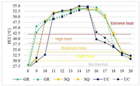
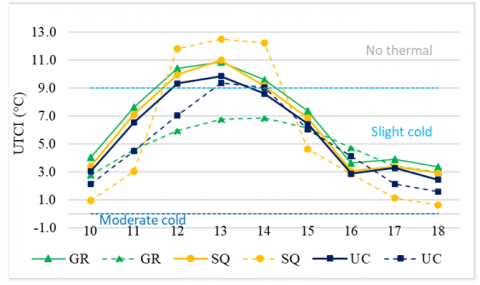
The simulation times to calculate thermal comfort conditions of the two tools are very different: from 15-20 minutes of SOLWEIG, to 9-11 hours with ENVI-met. In Table 5, the average values of UTCI and PET for August 7th (8 am-8 pm) and for January 1st (10 am-6 pm) are shown for the year 2015 (see Figure 2). The mean relative absolute error (MRAE) varies in summer from 0.03 to 5.34% and in winter from 1.63 to 37.76% and the main errors can be observed in wintertime and with UTCI; even if, in this case, the absolute errors are quite low (about 1-2℃).
Table 5. Thermal comfort analysis on three points of interest (ENVI-met and SOLWEIG comparison)
|
Districts |
Summer |
Winter |
||||||||||
|
|
PET (°C) |
UTCI (°C) |
PET (°C) |
UTCI (°C) |
||||||||
|
Mediterraneo |
GR |
SQ |
UC |
GR |
SQ |
UC |
GR |
SQ |
UC |
GR |
SQ |
UC |
|
ENVI-met |
45.29 |
44.70 |
42.14 |
39.77 |
39.00 |
38.54 |
2.12 |
2.46 |
1.99 |
4.78 |
5.35 |
4.07 |
|
SOLWEIG |
45.51 |
44.90 |
41.27 |
39.31 |
39.01 |
37.27 |
2.42 |
3.09 |
1.89 |
5.72 |
6.40 |
5.14 |
|
Arquata |
GR |
SQ |
UC |
GR |
SQ |
UC |
GR |
SQ |
UC |
GR |
SQ |
UC |
|
ENVI-met |
42.24 |
45.57 |
44.61 |
39.05 |
41.08 |
36.88 |
2.98 |
2.50 |
2.59 |
4.92 |
5.55 |
5.02 |
|
SOLWEIG |
40.45 |
44.72 |
43.86 |
36.97 |
38.94 |
38.52 |
3.46 |
2.98 |
2.55 |
6.78 |
6.28 |
5.83 |
Figure 3. Representation of SVF (a) and Tmrt (b) in the central District 1 of Turin on August 7th, 2015 at 1 p.m
(a)
(b)
Figure 4. SOLWEIG (solid line) and ENVI-met (dashed line): (a) Mediterraneo August 7th; (b) Arquata January 1st
Figure 4 shows the hourly results on the same points in the hot and cold days in the two neighborhoods. The graphs show similar trends with major errors with the UTCI index in winter.
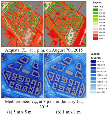
4.2 The influence of resolution at district and urban scale
The results of SOLWEIG were compared to describe the spatial distribution of the mean radiant temperature in the different districts and with another level of resolution: from 5 m x 5 m to 1m x 1m.
Figure 5. Tmrt with different cells’ grid resolutions
Figures 5 show a comparison between the output maps of Tmrt with 5 m and 1 m grids. The increased accuracy of the results increases the calculation time from 15-20 minutes to 1 hour, which is an adequate time for a neighborhood-scale simulation.
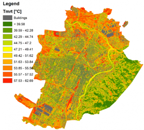
Finally, a first urban-scale analysis was conducted on the entire city of Turin on an area of about 130 km2 to observe the potential of SOLWEIG tool.
To calculate the SVF and Tmrtthe city has been divided into three main areas called A, B, and C as the software has a limit of 4,000,0000 cells (see Table 2). Then, the results of the three simulations with cells of 5m x 5m were aggregated to check the overall result at urban scale. Figures 6 show the average daily values of Tmrt from 10 a.m. to 6 p.m. in winter (a) and from 8 a.m. to 8 p.m. in summer (b).
(a) Average winter Tmrtfrom 10 am to 6 p.m.
(b) Average summer Tmrt from 8 am to 8 p.m.
Figure 6. Tmrt average values on January 1st and August 7th 2015 for the City of Turin (about 130 km2)
Table 6. Simulations times for the three areas in Turin
|
Turin |
Area |
Simulation times with SOLWEIG (h) |
|
|
areas |
(%) |
January 1st |
August 7th |
|
A |
29.69 |
9.32 |
10.54 |
|
B |
37.52 |
12.37 |
11.43 |
|
C |
32.79 |
12.19 |
11.17 |
Table 6 shows the three areas’ sizes and the simulation times to calculate the Tmrt with SOLWEIG for the city of Turin. It is possible to observe that, with this tool, it is possible to do thermal comfort analyses at urban scale with reasonable times of simulation. Then, PET and UTCI can be evaluated only in some points; plugins will likely be available soon for the calculation of thermal comfort indicators in all points.
Although previous work has focused on methods to assess outdoor thermal comfort in built environments, there has been little research on its evaluation at urban scale. In this work, SOLWEIG was compared with ENVI-met for thermal comfort analyses in various urban spaces in critical (i.e., hot and cold) weather conditions. Our research highlights the main differences between SOLWEIG and ENVI-met tools by analyzing the models used. The results of this work showed that SOLWEIG seems to be a more suitable tool since it offers the best compromise between simulation time and accuracy; especially for assessment and analyses at the urban scale, SOLWEIG allows to assess the overall impact of interventions for the mitigation of thermal comfort conditions at urban scale. ENVI-met is more useful for feasibility studies with a high spatial and temporal resolution, or for the pre-design phase of little neighborhoods. These results show a good similarity between ENVI-met and SOLWEIG; SOLWEIG has a good quality of accuracy despite the simplified assumptions used in the computational models. However, some limitations are noteworthy: forced meteorological data limit the accuracy, especially in winter conditions and with UTCI index. Future work will evaluate outdoor thermal comfort across the whole city in order to prioritize the interventions, identify critical areas and define the urban characteristics for more livability of outdoor spaces.
[1] Nastos, P.T., Matzarakis, A. (2012). The effect of air temperature and human thermal indices on mortality in Athens, Greece. Theoretical and Applied Climatology, 108: 591-599. https://doi.org/10.1007/s00704-011-0555-0
[2] Cochran, F.V., Brunsell, N.A. (2017). Biophysical metrics for detecting more sustainable urban forms at the global scale. International Journal of Sustainable Built Environment, 6(2): 372-388. https://doi.org/10.1016/j.ijsbe.2017.05.004
[3] Ahmadiana, E., Sodagara, B., Millsa, G., Byrda, H., Binghamb, C., Zolotasc, A. (2019). Sustainable cities: The relationships between urban built forms and density indicators. Cities, 95: 102382. https://doi.org/10.1016/j.cities.2019.06.013
[4] Lam, C.K.C., Lee, H., Yang, S., Park, S. (2021). A review on the significance and perspective of the numerical simulations of outdoor thermal environment. Sustainable Cities and Society, 71: 102971. https://doi.org/10.1016/j.scs.2021.102971
[5] Jänicke, B., Milošević, D., Manavvi, S. (2021). Review of user-friendly models to improve the urban micro-climate. Atmosphere, 12(10): 1291. https://doi.org/10.3390/atmos12101291
[6] Bruse, M., Fleer, H. (1988). Simulating surface–plant–air interactions inside urban environments with a three dimensional numerical model. Environmental Modelling Software, 13(3-4): 373-384. https://doi.org/10.1016/S1364-8152(98)00042-5
[7] Lindberg, F., Thorsson, S., Holmer, B. (2008). SOLWEIG 1.0 - Modelling spatial variations of 3D radiant fluxes and mean radiant temperature in complex urban settings. International Journal of Biometeorology, 52: 697-713. https://doi.org/10.1007/s00484-008-0162-7
[8] Thorsson, S., Lindberg, F., Björklund, J., Holmer, B., Rayner, D. (2010). Potential changes in outdoor thermal Ccomfort conditions in Gothenburg, Sweden due to climate change: The influence of urban geometry. International Journal of Climatology, 31: 324-335. https://doi.org/10.1002/joc.2231
[9] Lau, K.K., Ren, C., Ho, J., Ng, E. (2016). Numerical modelling of mean radiant temperature in high-density sub-tropical urban environment. Energy and Buildings, 114: 80-86. https://doi.org/10.1016/j.enbuild.2015.06.035
[10] Lindberg, F., Onomura, S., Grimmond, C.S.B. (2016). Influence of ground surface characteristics on the mean radiant temperature in urban areas, International Journal of Biometeorology, 60: 1439-1452. https://doi.org/10.1007/s00484-016-1135-x
[11] Thom, J.K., Coutts, A.M., Broadbent, A.M., Tapper, N.J. (2016). The influence of increasing tree cover on mean radiant temperature across a mixed development suburb in Adelaide, Australia. Urban Forestry & Urban Greening, 20: 233-242. https://doi.org/10.1016/j.ufug.2016.08.016
[12] Aminipouri, M., Knudby, A.J., Krayenhoff, E.S., Zickfeld, K., Middel, A. (2019). Modelling the impact of increased street tree cover on mean radiant temperature across Vancouver's local climate zones. Urban Forestry & Urban Greening, 39: 9-17. https://doi.org/10.1016/j.ufug.2019.01.016
[13] Aminipouri, M., Rayner, D., Lindberg, F., Thorsson, S., Knudby, A.J., Zickfeld, K., Middel, A., Krayenhoff, E.S. (2019). Urban tree planting to maintain outdoor thermal comfort under climate change: The case of Vancouver's local climate zones. Building and Environment, 158: 226-236. https://doi.org/10.1016/j.buildenv.2019.05.022
[14] Lindberg, F., Grimmond, C.S.B., Gabey, A., et al. (2018). Urban Multi-scale Environmental Predictor (UMEP): An integrated tool for city-based climate services. Environmental Modelling and Software, 99: 70-87. https://doi.org/10.1016/j.envsoft.2017.09.020
[15] Lindberg, F., Grimmond, C.S.B. (2011). The influence of vegetation and building morphology on shadow patterns and mean radiant temperatures in urban areas: Model development and evaluation. Theoretical and Applied Climatology, 105: 311-323. https://doi.org/10.1007/s00704-010-0382-8
[16] Rayman, AA.VV. Estimation and calculation of the mean radiant temperature within urban structures, https://www.urbanclimate.net/rayman/description.htm, accessed on May 2022.
[17] Reindl, D.T., Beckman, W.A., Duffie, J.A. (1990). Diffuse fraction correlations. Solar Energy, 45(1): 1-7. https://doi.org/10.1016/0038-092X(90)90060-P
[18] Gála, C., Kántor, N. (2020). Modeling mean radiant temperature in outdoor spaces: A comparative numerical simulation and validation study. Urban Climate, 32: 100571. https://doi.org/10.1016/j.uclim.2019.100571
[19] Hagemeier, M., Leuschner, C. (2019). Leaf and crown optical properties of five early-, mid- and late-successional temperate tree species and their relation to sapling light demand. Forests, 10(10): 925. https://doi.org/10.3390/f10100925
[20] Palomo Del Barrio, E. (1998). Analysis of the green roofs cooling potential in buildings. Energy and Buildings, 27(2): 179-193. https://doi.org/10.1016/S0378-7788(97)00029-7
[21] Jänicke, B., Meier, F., Hoelscher, M.T., Scherer, D. (2015). Evaluating the effects of façade greening on human bioclimate in a complex urban environment. Advances in Meteorology, 2015: 747259. https://doi.org/10.1155/2015/747259
[22] Hu, S., Yan, D., Azar, E., Guo, F. (2020). A systematic review of occupant behavior in building energy policy. Building and Environment, 175: 106789. https://doi.org/10.1016/j.buildenv.2020.106807
[23] Mutani, G., Todeschi, V. (2021). Roof-integrated green technologies, energy saving and outdoor thermal comfort: Insights from a case study in urban environment. International Journal of Sustainable Development and Planning, 16(1): 13-23. https://doi.org/10.18280/ijsdp.160102
[24] Mutani, G., Todeschi, V., Beltramino, S. (2022). Improving outdoor thermal comfort in built environment assessing the impact of urban form and vegetation. International Journal of Heat and Technology, 40(1): 23-31. https://doi.org/10.18280/ijht.400104
[25] Redon, E.C., Lemonsu, A., Masson, V., Morille, B., Musy, M. (2017). Implementation of street trees within the solar radiative exchange parameterization of TEB in SURFEX v8.0. Geoscientific Model Development, 10: 385-411. https://doi.org/10.5194/gmd-10-385-2017