Tat Thang Nguyen
© 2021 IIETA. This article is published by IIETA and is licensed under the CC BY 4.0 license (http://creativecommons.org/licenses/by/4.0/).
OPEN ACCESS
The drift-flux model is widely used in study, calculation and design of two-phase flow. It is a highly efficient model that requires little computation resources. In the model, accurate calculation of the distribution parameter C0 and the drift velocity Vgj is a critically important factor. The calculation requires simultaneously measured data of phase velocity and void fraction distributions or profiles. By using currently widely used methods for two-phase flow measurement, satisfying the requirement is highly difficult. This paper presents novel results of simultaneous measurement of the phase velocity and void fraction profiles in a vertical round tube of 50 mm inner diameter. A combination measurement method has been developed. It comprises the multiwave Ultrasonic Velocity Profile (multiwave UVP) method and the Wire Mesh Tomography (WMT). Based on the measured data, C0 and Vgj have been calculated. They have been compared with those of the published experimental data and correlations. Analyses of the measured data have been carried out. For the first time, the analysis results reveal the variation of C0 and Vgj in the measured flow conditions. More importantly, the data obtained are also useful for the development and validation of the computational codes for two-phase flow.
drift flux model, Ultrasonic Velocity Profiling - UVP, Wire Mesh Tomography – WMT, two-phase flow, simultaneous measurement, velocity distribution, void fraction distribution
Void fraction that is also known as the gas hold-up or the volumetric concentration of the gas phase in gas-liquid two-phase flows is a critically important parameter in the design and operation of the thermal hydraulic systems in, for example, various nuclear power reactor [1], solar dynamics space station - SDPSS [2], oil and gas gathering and transportation [3]. One of the reasons is that it directly and critically affects the flow regimes and hence the heat transfer characteristics and/or the efficiency of the systems [4]. For instance, in boiling water nuclear reactors, the nuclear reactivity that has decisive effect on the reactor power depends directly on the void fraction parameter. Hence the safe and optimal design/operation of the systems essentially rely on the accurate knowledge of the void fraction parameter in the systems. The drift-flux model was developed as a highly efficient tool either for predicting the void fraction parameter or analyzing and interpreting the experimental data [5].
The drift-flux model is widely used in various nuclear thermal hydraulic simulation codes (e.g., RELAP5, etc.) [6] and also in CFD - Computational Fluid Dynamics codes (e.g., Ansys FLUENT) [7]. The model includes two important parameters, i.e., the distribution parameter C0 and the drift velocity Vgj. The former takes into account the effects of the void fraction and of the mixture volumetric flux profiles. The latter considers the effects of the local relative velocity between the gas phase and the two-phase mixture [5, 6]. The two parameters depend on various factors such as the flow pattern, geometry, channel size, bubble size of the gas phase, etc. When the 1-dimensional (1D) average values of the two-phase flow parameters (e.g., void fraction, phase velocities) are used, the calculation of C0 and Vgj cannot take into consideration these effects. Besides experimental measurements, different empirical correlations have been developed and commonly adopted to calculate the two parameters [6]. In order to verify the accuracy of these correlations in different flow conditions, experimental data in the form of profiles (i.e., distributions) of the phase parameters (simultaneously measured data) are requested. Zuber and Findlay, 1965 [5] clearly recommended that “The results of this analysis indicate that, for a detailed understanding of the phenomenon, simultaneously recorded data on both the flow and concentration profiles are required”. In the general context of two-phase flow, the flow and concentration profiles here mean the profiles of phase velocities and void fraction. Consequently, the simultaneously measured data of two-phase flow are of immense importance.
Experimental methods for simultaneous measurements of void fraction and phase velocity profiles in two-phase flow recently still have limitations. Generally, void fraction measurement methods (e.g., the ones that are based on using optics, radiation, or measuring probe, etc.) are not able to measure phase velocity distributions and vice versa. Moreover, few methods can measure instantaneous profiles (of either void fraction or phase velocities) in two-phase flows (e.g., see [8] for a recent review of two-phase flow measurement methods). Some previous studies have been successfully carried out to measure simultaneously the two-phase flow parameters by using a combination measurement method (e.g., see [9, 10]). The void fraction profile was measured by the optical method that would be applicable only to low void fraction flow conditions in order to avoid the bubble overlapping in the flow images. The velocity distributions of liquid and bubbles were measured by using the UVP method. The phase separation technique in these studies required a difference between the velocities of the bubble phase and the liquid phase. Therefore, the applicability of these methods to different flow configurations (two-phase flow in the horizontal direction, for example) would be limited. In gas-liquid two-phase flow in horizontal direction, generally, there would be no (or very small) difference between the velocities of the two phases.
The WMT method, though intrusive, is highly useful for the measurement of 2-dimensional (2D) cross-sectional void fraction distribution of two-phase flows [11]. It can measure instantaneous void fraction profile of two-phase flows at considerably high measurement frequency (a very high frequency up to 10 kHz has been achieved [11]). Besides, the multiwave UVP method has recently been developed to be a powerful method that enables simultaneous and separate measurement of the velocity profiles of bubbles and liquid in bubbly two-phase flow [12, 13]. By applying both WMT and multiwave UVP measurements at the same time and at the same measurement location, simultaneous measurement of two-phase flow parameters can be obtained [14-16].
Among various important applications of gas-liquid two-phase flows, bubbly counter current flow plays critical roles in different areas of industry including chemistry, petroleum production, food production, nuclear power generation etc. [17-19]. Consequently, simultaneous measurement of the flow is of significant interest. Measured data can be useful for different purposes including theoretical study of two-phase flow as well as development of computational codes etc.
Taking into account the fact that simultaneously measured profile data of multiphase flow parameters are still lacking, the objectives of this study are to:
The analyses fully take into account the 2D effects of the void fraction and phase velocity profiles. The received results can be useful for both experimental investigations and numerical simulations of two-phase flow in general and of counter-current bubbly flow in a vertical pipe in particular.
2.1 Basic equations
The 1D drift-flux model was originally developed by Zuber and Findlay, 1965 [5]. In order to derive the model’s equations, first, it is necessary to introduce the formulation of the average value of a scalar or of a vector quantity X over the cross-sectional area of the flow (e.g., pipe or channel) as shown in Eq. (1) below:
$\left\langle X \right\rangle =\left( 1/A \right)\int_{A}{XdA}$ (1)
where, A is the area of the cross-section of the flow.
The drift velocity Vgj of the gas phase, which is defined as the difference between the velocity of the gas phase and the volumetric flux density of the two-phase mixture, is shown in Eq. (2) below:
Vgj = vg – j (2)
where, vg is the velocity of the gas phase in the two-phase flow; j is the volumetric flux density of the two-phase mixture which is defined by j = jl + jg; where jl = (1-α)vl; jg = αvg; α is the void fraction which is also known as the volumetric concentration of the gas phase.
By using the definition of jg and Eq. (2), the expression of the average value of vg is given by
$\left\langle {{v}_{g}} \right\rangle =\left\langle {{j}_{g}}/\alpha \right\rangle =\left\langle j \right\rangle +\left\langle {{V}_{gj}} \right\rangle $ (3)
Though, to some extent, Eq. (3) can be useful in the analyses of two-phase flow systems, the consideration of the gas volumetric flux density jg, as shown in Eq. (4), instead of the gas velocity vg, can be more advantageous and convenient [5].
$\left\langle {{j}_{g}} \right\rangle =\left\langle \alpha {{v}_{g}} \right\rangle ={{Q}_{g}}/A$ (4)
In the published literature, this quantity is widely used and commonly denoted by “superficial velocity”.
From the above relations, the definition of the void-fraction-weighted mean-value of the quantity X comes naturally as shown in Eq. (5).
$\overline{X}=\left\langle \alpha X \right\rangle /\left\langle \alpha \right\rangle =\left( (1/A)\int_{A}{\alpha XdA} \right)/\left( (1/A)\int_{A}{\alpha dA} \right)$ (5)
As a result, the void-fraction-weighted mean-velocity $\overline{{{v}_{g}}}$ of the gas phase can be obtained as shown in Eq. (6).
$\overline{{{v}_{g}}}=\left\langle \alpha {{v}_{g}} \right\rangle /\left\langle \alpha \right\rangle =\left\langle {{j}_{g}} \right\rangle /\left\langle \alpha \right\rangle $ (6)
As mentioned by Zuber and Findlay [5], this definition is the same as that of the mean velocity of particles described in the kinetic theory of gases and liquids. Based on Eq. (2) and Eq. (5), the void-fraction-weighted mean-velocity of the gas phase vg can also be written as:
$\overline{{{v}_{g}}}=\left\langle \alpha j \right\rangle /\left\langle \alpha \right\rangle +\left\langle \alpha {{V}_{gj}} \right\rangle /\left\langle \alpha \right\rangle $ (7)
Apparently, it is worth noting here that the average velocity <vg> described by Eq. (3) and the void-fraction-weighted mean-velocity $\overline{{{v}_{g}}}$ shown in Eq. (6) and Eq. (7) express the same flow parameter but are formulated in different ways [5].
The weighted mean velocity $\overline{{{v}_{g}}}$ of the gas phase, indicated by Eq. (7), can be re-written in several forms, e.g., the one shown in Eq. (8), which can be highly useful to analyze the experimentally measured data and to determine the average void fraction $\left\langle \alpha \right\rangle $, provided that C0 and Vgj in Eq. (8) are known. Thus, by manipulating Eq. (7), we can derive:
$\overline{{{v}_{g}}}=\left\langle {{j}_{g}} \right\rangle /\left\langle \alpha \right\rangle ={{C}_{0}}\left\langle j \right\rangle +\left\langle \alpha {{V}_{gj}} \right\rangle /\left\langle \alpha \right\rangle $ (8)
where the distribution parameter C0 is defined by:
$C_{0}=\frac{\langle\alpha j\rangle}{\langle\alpha\rangle\langle j\rangle}=\frac{(1 / A) \int_{A}^{-} \alpha j d A}{\left((1 / A) \int_{A}^{\operatorname{L}} \alpha d A\right)\left((1 / A) \int_{A}^{\operatorname{l}} j d A\right)}$ (9)
2.2 Main characteristics
Eq. (8) can be used to analyze any two-phase flow regime [5]. Furthermore, Eq. (8) takes into consideration both the effect of nonuniform flow and void fraction profiles, and also the effect of the local relative velocity between the gas phase and the two-phase mixture.
The first effect is taken into account by the distribution parameter C0. The second effect is considered by using the weighted mean drift velocity <αVgj>/<α>. For each specific flow regime, the value of the average void fraction <α> can be obtained from Eq. (8) by choosing the suitable velocity (flux) and void fraction profiles, and the appropriate value of the drift velocity.
As suggested by Zuber and Findlay [5], the value of C0 should be:
3.1 Experimental apparatus
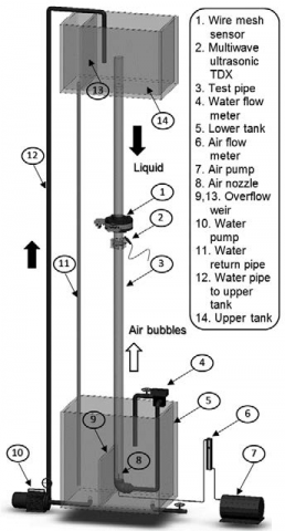
The experimental flow loop of the air-water counter-current bubbly flow in a vertical pipe is depicted in Figure 1. The apparatus was also used in the related studies of WMT and multiwave UVP measurement for two-phase flows. Multiwave UVP method is based on using ultrasound (of two basic ultrasonic frequencies 2 and 8 MHz) to measure phase velocities. So the method is non-intrusive and non-invasive. More importantly, the method is capable of measuring instantaneous velocity profiles of the bubble phase and liquid phase. WMT is an intrusive measurement method that uses two electrical conductivity sensor arrays. It is basically an electrical conductivity probe with capability of measuring 2D void fraction distribution of the flow field. For more details, interested readers can refer to, e.g., [16].
As presented in Figure 1, a counter-current bubbly flow was generated in the vertical test pipe (3) made of transparent acrylic that enables optical visualization of the flow field. The inner diameter (D) and the length of the test pipe were 50 mm and 2745 mm, respectively. Water flowed downward in the test pipe due to the gravity effect. The water flowrate in the test pipe was measured by using the flowmeter (4). It could be adjusted by using a needle valve located at the outlet of the pipe. Air bubbles were generated at the bottom of the pipe by using the air nozzle (8). The air nozzle was an air stone attached to the outlet of the supply gas pipe. Bubbles rose upward in the test pipe, due to the buoyancy effect. Hence a counter-current bubbly flow was generated. Air bubbles of almost uniform diameter in the range 2 - 3 mm were observed in the experiments. The air flowrate was measured and controlled by using the float flow meter (6). It is worth noting here that the bubbly flow regime occurred in the whole length of the working pipe. There was no change in the two-phase flow regime in the pipe.
To measure the cross-sectional void fraction profile, the wire mesh sensor (WMS) (1) was used. It was located at the downstream side (based on the air flow direction) of the multiwave ultrasonic sensor (2).
Hence the measurement positions of both WMT and multiwave UVP methods could be considered to be at the same position that was at 21D from the water inlet, and 34D from the air inlet. According to previous published results (e.g., see [13, 14, 16]), the two-phase flow field is well-developed and is stable. For details of the WMT and multiwave UVP methods for two-phase flow measurement, interested readers are referred to [13, 16].
Figure 1. Bubbly counter-current flow loop and experimental setup
3.2 Experimental conditions and measurement settings
The Reynolds numbers Rel and Reg of the water and bubble phases, respectively, are defined in Eq. (10) and Eq. (11). They suggest some idea of the flow regimes of each phase.
Rel = jlD/νl (10)
Reg = jgD/νg (11)
where, νl and νg are the kinematic viscosity of water and air, respectively.
The experimental conditions of the counter-current air-water bubbly flow is introduced in Table 1. The minus sign implies the downward direction as opposed to the upward direction which has a positive sign.
Table 1. Experimental conditions
|
Parameter |
Range |
|
Superficial velocity of water - jl [mm/s] |
-10 |
|
Reynolds number of the water phase - Rel [-] |
-500 |
|
Superficial velocity of air - jg [mm/s] |
1 to 8 |
|
Bubble diameter [mm] |
2 to 3 |
|
Reynolds number of the gas flow - Reg [-] |
3.3 to 26.5 |
|
Water temperature [℃] |
25 |
The measurement settings of both WMT and multiwave UVP methods are tabulated in Table 2.
Table 2. Measurement settings
|
Parameter |
Range |
|
WMT measurement frequency [Hz] |
10,000 |
|
Temporal resolution [ms] |
0.1 |
|
Spatial resolution of the WMT measurement in the 2D cross-sectional plane [mm] |
3 × 3 |
|
Spatial resolution of the WMT measurement in the flow direction (i.e. vertical direction) [mm] |
1.5 |
|
Maximum measurable velocity (in the WMT method) of the gas phase [m/s] |
15 |
|
Basic ultrasonic frequencies of the multiwave UVP method [MHz] |
2 and 8 |
|
Spatial resolution of UVP measurement by 2 and 8 MHz frequencies [mm] |
0.74 |
|
Maximum measurable velocity (in the UVP method) of 2 and 8 MHz sensors [m/s] |
2.1 and 0.52 |
|
Temporal resolution of 2 and 8 MHz frequencies [ms] |
16 |
|
Sound speed in water [m/s] |
1480 |
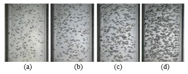
Figure 2 below shows typical images of the stable flow field corresponding to the flow conditions jl = -10 mm/s and jg = 1, 2, 4, 8 mm/s from left to right, respectively. The images were obtained by using a PHOTRON FASTCAM high speed camera (Photron Inc.) which is capable of taking images at the maximum speed of 500,000 fps (frames per second). The actual imaging speed used was set based on the lighting condition. The quality of the flow images was sufficiently high as can be observed, e.g., in Figure 2, visually. There appears no blur around the bubble edge as well as no streak in the bubble movement.
Figure 2. Typical flow images corresponding to jl = -10 mm/s and jg = 1, 2, 4, 8 mm/s
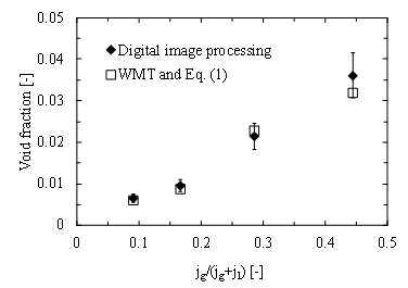
The average void fraction calculated by using the WMT measured data was further confirmed by comparing it with that obtained by analyzing the recorded flow images. Figure 3 presents the measured data of the void fraction against the non-dimensionalized gas influx. The non-dimensionalized gas influx was systematically used throughout this study to characterize the measurement conditions. In addition, in Figure 3, an error bar that shows an error amount of 15% of the void fraction measured by digital image processing is presented. As illustrated in Figure 3, at the high-void-fraction end, the evaluation of the void fraction using the flow images would include somewhat larger error than in other cases. The main reason would have been the decreased accuracy of the void fraction estimated by digital image processing in this case. As depicted in Figure 2 (d), some bubbles appear to overlap each other in the flow image, which makes digital image processing encounter lower accuracy.
Figure 3. Averaged void fractions measured by WMT and digital image processing at the measurement location (The error bar shows an error amount of 15%.)
3.3 Measurement error
The accuracy of void fraction measurement by WMT has been well confirmed to be sufficiently high in both previous studies [11, 20] and in this investigation. In general, the error of WMT measurement of void fraction has been reported to be less than 10% by comparing WMT measured data with that of either gamma-densitometry or digital image processing. The same behavior has also been confirmed in this study.
The high accuracy of the multiwave UVP method has also been addressed in related studies (e.g. see [12-16]). The measurement errors of the liquid phase and of the bubble phase can be as low as less than 1% (e.g. see [21]).
3.4 Measured data of the simultaneous distributions of the phase velocities and void fraction
As depicted above, the data of the void fraction measured by WMT method have been compared with the results of optical visualization and digital image processing. Fairly good agreement between the two data was always secured for all flow conditions. Hence, the WMT measured data of void fraction should be of acceptably high quality. The high accuracy of the results of the phase velocities measured by the multiwave UVP method was well confirmed in the previous study [13-15]. Consequently, the use of the measured data of the flow and void fraction distributions in the analyses in the next parts of this paper would be straightforward.
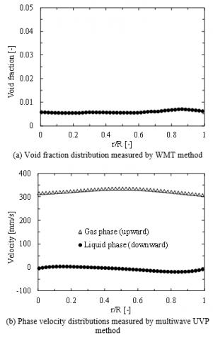
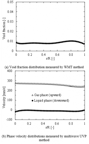
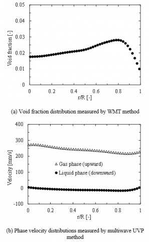
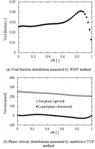
Figures 4 to 7 below present the measured data by WMT and multiwave UVP method for the flow conditions presented in Figure 2. As seen in the figures, the measured profiles of void fraction exhibit the tendency of moving from constant-void fraction profile regime to the intermediate-peak regime [16, 22]. Based on the measured data, analyses of the drift-flux model parameters have been carried out later on in the next chapter in this paper. It would be worth noting also that the measured data or the experimental data set shown in this section would be of significant interest for the development and validation of numerical models (or CFD models) of two-phase flow.
Figure 4. Measured data along a pipe radius (r/R = 0: pipe center; r/R = 1: pipe wall) when jl = -10 mm/s and jg = 1 mm/s
Figure 5. Measured data along a pipe radius (r/R = 0: pipe center; r/R = 1: pipe wall) when jl = -10 mm/s and jg = 2 mm/s
Figure 6. Measured data along a pipe radius (r/R = 0: pipe center; r/R = 1: pipe wall) when jl = -10 mm/s and jg = 4 mm/s
Figure 7. Measured data along a pipe radius (r/R = 0: pipe center; r/R = 1: pipe wall) when jl = -10 mm/s and jg = 8 mm/s
As predicted [5], the distribution parameter C0 is expected to be in the range from 1.0 to 1.5 in the flow regime investigated in this study. As seen in Figures 4 to 7, the void fraction profiles would vary from a constant profile to the one that has higher void fraction near the pipe wall than that at the pipe center.
4.1 Distribution parameter C0
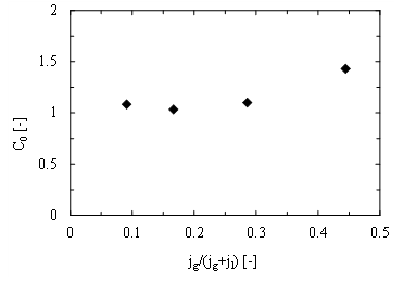
Based on the simultaneously measured data of the void fraction and phase velocity distributions, the distribution parameter C0 can be calculated by using Eq. (8). As depicted in Figure 8, the derived value of C0 (by using the measured data presented in Figures 4 to 7) has been found to well belong to the range 1 - 1.5. The received result of this study shows good accord with the range of C0 predicted theoretically by Zuber and Findlay, 1965 [5]. Previously, when only cross-sectional average void fraction was used, attention was not adequately given to the detailed void fraction profile (i.e. the concentration profile as mentioned in the Ref. [5]).
It would be worth mentioning that the result obtained here is for the counter-current air-water bubbly flow in a vertical pipe of 50 mm inner diameter. There exist calculated data of C0 found in the published literature for the counter-current air-water bubbly flow but in a vertical rectangular channel [9]. The result presented in the Ref. [9] was found to be very close to 1.0 which is in reasonable agreement with what has been found in this study for counter-current bubbly flow in a vertical round tube.
In general, the calculated data of C0 in this study has fully taken into account the distributions of flow parameters rather than a representative value averaged over the cross-section of the pipe. The accuracy of the estimation of C0 is therefore believed to be well improved. Particularly, as depicted in Figure 8, the effect of the void fraction distribution appears to be remarkable. The void fraction profile shown in Figure 7 (a) for the measurement condition jg = 8 mm/s is essentially different from those obtained at low gas influx jg. C0 in this case approaches very close to 1.5.
Figure 8. Distribution parameter C0 experimentally evaluated based on the simultaneously measured data
4.2 Drift velocity Vgj
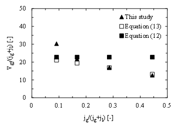
By using the simultaneously measured data of the void fraction and phase velocity profiles, the drift velocity Vgj of the bubble phase relative to the mixture velocity has also been calculated. Based on Eq. (2) with some manipulations, results of the estimation of Vgj have been obtained and presented in Figure 9 for the flow conditions investigated.
By using the correlation in Eq. (12), which was proposed by Zuber and Findlay, 1965 [5], the predicted drift velocity in the flow conditions was also available. It is worth noting that in Eq. (12), the effect of void fraction, which would be of critical importance, is completely not taken into account in the prediction of Vgj. Consequently, using Eq. (12), a constant value of Vgj is derived and also shown in Figure 9. Nevertheless, as seen in Figure 9, the predicted value of Vgj falls in the middle of the range of Vgj calculated in this study. This also would suggest the averaging nature of Eq. (12).
$V_{g j}=v_{g}-j=1.53\left(\sigma g \Delta \rho / \rho_{l}^{2}\right)^{1 / 4}$ (12)
where, σ is the surface tension of water; g is the gravitational acceleration; ∆ρ = ρl - ρg; ρl is the water density; ρg is the air density.
In addition, another widely used correlation for drift velocity calculation is also used [23]. In contrast to Eq. (12), in Eq. (13), the effect of void fraction is considered in the prediction of Vgj. This would suggest that the accuracy of the prediction is improved accordingly. In fact, this is confirmed as shown in Figure 9.
$V_{g j}=v_{g}-j=\sqrt{2}\left(\sigma g \Delta \rho / \rho_{l}^{2}\right)^{1 / 4}(1-<\alpha>)^{1.75}$ (13)
Using Eq. (13), the value of Vgj has been obtained for the flow conditions investigated. Interestingly, when void fraction is taken into account in Eq. (13), the experimentally calculated drift velocity in this study appears to fit well with that of the correlation over most of the investigated flow conditions. There exists discrepancy between the two results toward the low end of the superficial gas influx jg. As expected, at low jg, void fraction becomes small. Accordingly, its effect in Eq. (13) becomes small. Hence, Vgj estimated by using Eq. (13) approaches that estimated by using Eq. (12), which would be the average value of Vgj.
In addition, compared with the calculated drift velocity of this study, the value Vgj = 0.231 m/s calculated by Aritomi et al., 1996 [9] for a different flow condition of the counter-current air-water bubbly flow in a vertical rectangular channel would also fall in the middle of the value range as can be seen in Figure 9.
Figure 9. Drift velocity Vgj experimentally evaluated based on the simultaneously measured data of the distribution of the multiphase flow parameters
In order to accurately estimate the parameters of the drift-flux model that is widely used in various numerical codes for two-phase flow simulation, novel simultaneous measurements of the void fraction and phase velocity profiles were carried out in this study. The counter-current air-water bubbly flow in a vertical pipe was measured. By using the drift-flux model’s equations, analyses of the measured data were performed. The following concluding remarks have been obtained.
|
X |
any scalar or vector quantity over a cross sectional area of the two-phase flow under investigation |
|
A |
area, m2 |
|
v |
velocity, m.s-1 |
|
j V |
volumetric flux density, m.s-1 drift velocity, m.s-1 |
|
Q |
phase volumetric flow rate, m3.s-1 |
|
C0 |
distribution parameter, [-] |
|
Re |
Reynolds number, [-] |
|
D |
pipe inner diameter, [m] |
|
g |
gravitational acceleration, m.s-2 |
|
Greek symbols |
|
|
$\alpha$ |
void fraction, [-] |
|
ν |
phase kinematic viscosity, m2.s-1 |
|
σ |
surface tension of the water, N.m-1 |
|
ρ |
phase density, kg.m-3 |
|
Subscripts |
|
|
g |
gas phase |
|
l |
liquid phase |
[1] Ishii, M., Hibiki, T. (2010). Thermo-Fluid Dynamics of Two-Phase Flow. Springer Science & Business Media. http://dx.doi.org/10.1007/978-1-4419-7985-8
[2] Song, H., Zhang, W., Li, Y., Yang, Z., Ming, A. (2016). Simulation of the vapor-liquid two-phase flow of evaporation and condensation. International Journal of Heat and Technology, 34(4): 663-670. http://dx.doi.org/10.18280/ijht.340416
[3] Luo, W., Li, Y., Wang, Q.H., Li, J.L., Liao, R.Q., Liu, Z.L. (2016). Experimental study of gas-liquid two-phase flow for high velocity in inclined medium size tube and verification of pressure calculation methods. Int. J. Heat Technol, 34(3): 455-464. https://doi.org/10.18280/ijht.340315
[4] Thome, J.R. (2006). Wolverine Engineering Databook III. Wolverine Tube, Inc.
[5] Zuber, N., Findlay, J.A. (1965). Average volumetric concentration in two-phase flow systems. Journal of Heat Transfer, 87: 453-468. https://doi.org/10.1115/1.3689137
[6] Ozaki, T., Hibiki, T. (2015). Drift-flux model for rod bundle geometry. Progress in Nuclear Energy, 83: 229-247. https://doi.org/10.1016/j.pnucene.2015.03.015
[7] ANSYS FLUENT (2011). Theory Guide, ANSYS Inc.
[8] Lee, Y.G., Won, W.Y., Lee, B.A., Kim, S. (2017). A dual conductance sensor for simultaneous measurement of void fraction and structure velocity of downward two-phase flow in a slightly inclined pipe. Sensors, 17(5): 1063. https://doi.org/10.3390/s17051063
[9] Aritomi, M., Zhou, S., Nakajima, M., Takeda, Y., Mori, M. (1997). Measurement system of bubbly flow using ultrasonic velocity profile monitor and video data processing unit, (II) flow characteristics of bubbly counter-current flow. Journal of Nuclear Science and Technology, 34(8): 783-791. https://doi.org/10.1080/18811248.1997.9733742
[10] Zhou, S., Suzuki, Y., Aritomi, M., Matsuzaki, M., Takeda, Y., Mori, M. (1998). Measurement system of bubbly flow using ultrasonic velocity profile monitor and video data processing unit, (III) comparison of flow characteristics between bubbly co-current and counter-current flows. Journal of Nuclear Science and Technology, 35(5): 335-343. https://doi.org/10.1080/18811248.1998.9733869
[11] Prasser, H.M., Böttger, A., Zschau, J. (1998). A new electrode-mesh tomograph for gas-liquid flows. Flow Measurement and Instrumentation, 9(2): 111-119. https://doi.org/10.1016/S0955-5986(98)00015-6
[12] Murakawa, H., Kikura, H., Aritomi, M. (2008). Application of ultrasonic multi-wave method for two-phase bubbly and slug flows. Flow Measurement and Instrumentation, 19(3): 205-213. https://doi.org/10.1016/j.flowmeasinst.2007.06.010
[13] Nguyen T.T., Murakawa H., Tsuzuki N., Kikura H. (2013). Development of multiwave method using ultrasonic pulse Doppler method for measuring two-phase flow. Journal of Japan Society of Experimental Mechanics, 13(3): 277-284. https://doi.org/10.11395/jjsem.13.277
[14] Nguyen, T.T. (2016). Study of ultrasonic velocity profiling method on boiling two-phase flow. PhD thesis, Tokyo Institute of Technology, Tokyo, Japan. LINK: http://t2r2.star.titech.ac.jp/rrws/file/CTT100708830/ATD100000413/.
[15] Nguyen, T.T. (2021). Evaluation of the effect of the concentration of seeding particles on spike-excitation doppler UVP measurement. Vietnam Journal of Mechanics, 43(1): 1-15. https://doi.org/10.15625/0866-7136/15554
[16] Nguyen, T.T., Kikura, H., Murakawa, H., Tsuzuki, N. (2015). Measurement of bubbly two-phase flow in vertical pipe using multiwave ultrasonic pulsed Dopller method and wire mesh tomography. Energy Procedia, 71: 337-351. https://doi.org/10.1016/j.egypro.2014.11.887
[17] Besagni, G., Inzoli, F. (2016). Influence of internals on counter-current bubble column hydrodynamics: Holdup, flow regime transition and local flow properties. Chemical Engineering Science, 145: 162-180. https://doi.org/10.1016/j.ces.2016.02.019
[18] Sukamta, S., Firdaus, R.A., Thoharudin, T. (2018). The characteristic of two-phase flow pattern on air-water countercurrent flow in vertical pipe. Key Engineering Materials, 792: 190-194. https://doi.org/10.4028/www.scientific.net/KEM.792.190
[19] Besagni, G., Inzoli, F., Ziegenhein, T. (2018). Two-phase bubble columns: A comprehensive review. ChemEngineering, 2(2): 13. https://doi.org/10.3390/chemengineering2020013
[20] Rahiman, M.H.F., Siow, L.T., Rahim, R.A., Zakaria, Z., Ang, V. (2015). Initial study of a wire mesh tomography sensor for liquid/gas component investigation. Journal of Electrical Engineering and Technology, 10(5): 2205-2210. https://doi.org/10.5370/JEET.2015.10.5.2205
[21] Nguyen, T.T., Murakawa, H., Tsuzuki, N., Duong, H.N., Kikura, H. (2016). Ultrasonic Doppler velocity profile measurement of single-and two-phase flows using spike excitation. Experimental Techniques, 40(4): 1235-1248. https://doi.org/10.1111/ext.12165
[22] Serizawa A, Kataoka I. (1988). Phase distribution in two-phase flow. In: Afgan N.H., Ed., Transient Phenomena in Multiphase Flow, Washington, DC, USA: Hemisphere, 1: 179-224. BOOK ISBN: 0891166823, 9780891166825
[23] Hibiki, T., Ishii, M. (2003). One-dimensional drift-flux model and constitutive equations for relative motion between phases in various two-phase flow regimes. International Journal of Heat and Mass Transfer, 46(25): 4935-4948. https://doi.org/10.1016/S0017-9310(03)00322-3