Abderrahim Mokhefi* | Mohamed Bouanini | Mohammed Elmir
© 2021 IIETA. This article is published by IIETA and is licensed under the CC BY 4.0 license (http://creativecommons.org/licenses/by/4.0/).
OPEN ACCESS
The purpose of research presented in this paper is to study the thermal and hydrodynamic effect of the non-isothermal laminar flow of a Al2O3-water nanofluid having shear thinning behavior in a mechanically stirred tank using the finite element method. Numerical simulation has been performed for a non-stationary two-dimensional flow controlled by certain influencing parameters such as the Reynolds number (1 ≤ Re ≤ 200), the behavior index (0.6 ≤ n ≤ 1) and the volume fraction of the alumina nanoparticles (0 ≤ φ ≤ 0.1). The simulation results obtained show that the addition of the Al2O3 nanoparticles in the base fluid leads to a significant enhancement in the heat transfer in the stirred tank compared to the base fluid. On the other hand, we note a slight decrease in the heat transfer with the decrease in the behavior index. It has also been noted, that the agitation power increases relatively with the volume fraction of the Alumina nanoparticles.
agitated tank, nanofluid, shear thinning, power consumption, heat transfer, laminar flow
The flow of complex fluids in the tanks provided with a rotary mobile is due to a unit operation called mechanical agitation. It presents a very important process for many industrial activities, notably in the pharmaceutical, petrochemical and food industry, it essentially contributes to the homogeneity of the mixture, or to the acceleration of various reactions. In addition to the uses of mechanical agitation in the hydrodynamic activities, this process plays a good role in the heat transfer through the heated vessel wall, in particular for the acceleration of chemical reactions or through heat exchangers in coiled agitated vessels. Given this mentioned importance, many researchers have submitted numerical simulations and experimental work related to hydrodynamic and thermal behavior in mechanically agitated tanks, in the presence of different types of agitators and different theologies of fluid, in order to improve the characteristics associated with optimal efficiency in thermo-hydrodynamics. Among the first researchers to have carried out this type of work, Bertrand et al. [1-3] who introduced a set of experimental work and numerical simulations in agitated tanks equipped with mobiles: tow-blade, anchor and barrier. They determined the characteristics of the flow and thermal behavior generated by these agitators for different theologies of non-Newtonian shear thinning fluid. Baccar et al. [4] have given a numerical hydrodynamic and thermal study of the turbulent flows induced in a closed cylindrical tank, provided with a six-blade radial turbine, they noted a strong contribution of the turbulent flows to the parietal heat transfer, giving place at the uniformity of the temperature field. Hami et al. [5] carried out a study, on the flow field and on the thermal profile generated by mechanical agitation, of a viscous fluid, in a vessel equipped with an inclined blades anchor. They noted an increase in the power consumption compared to the case of the anchor with straight blades, on the other hand, a decrease in Nusselt number. Rahmani et al. [6] studied by numerical voice, the viscoplastic behavior of the mechanical agitation in a tank equipped with a barrier, where they noted a quasi-immobilization of the fluid inside the agitated system. Benmoussa and Rahmani [7] have described in depth numerical study of the hydrodynamic and the thermal behavior in stirred tank, filled with a yield stress fluid with regularization model of Bercovier and Engelman. They found that the thermal performance is intimately related to the hydrodynamics state of the entire stirred tank. In the context of improving hydrodynamic efficiency in agitated tanks, numerical studies, of mechanical agitation have been presented by Ameur et al. [8, 9], of the hydrodynamic characteristics in presence of non-Newtonian fluids in a tank provided with a Maxblend impeller and the other with a straight blade anchor.
The process of enhancement of convective heat transfer has received a lot of attention from researchers in this domain. This can be achieved by increasing the exchange surface with the fluid or by using of microscopic channels, as well as by the using of fluids known for more efficient heat transfer like water and glycol. Among these fluids, nanofluids are one of the most important substances used to improve heat transfer. Nanofluids are very present in the work to improve heat transfer in various industrial fields.
They are characterized by their high thermal conductivities coefficient compared to those of conventional fluids. The preparation of this type of fluid consists in suspending a moderate concentration of metallic particles with diameters between 1 and 100 nm in a base fluid. Since Choi [10] introduced the notion of nanofluids in the literature on fluid dynamics [11], several experimental works and numerical simulations have been carried out in order to determine their properties and their reliability in various industrial activities [12-14]. The use of nanofluids in mechanical agitation in order to heat other fluids in exchangers with rotating mobile has been present. Perarasu et al. [15, 16] conducted a comparative study on improving heat transfer using a nanofluid in a spirally agitated container. They found that the heat transfer coefficient of nanofluid turns out to be higher than that of water and increases with increasing volume concentrations. Srinivas et al. [17] studied the performance of a stirred helical coil heat exchanger using an Al2O3-water nanofluid in terms of energy consumed to heat another fluid. They observed that increasing the agitator speed and the fluid temperature also resulted in more energy savings. Similar work has been carried out by Naik et al. [18]. The latter however took into account the rheology of the nanofluid in the non-Newtonian case (Alumina/CMC). They have shown experimentally that the heat transfer performance of non-Newtonian nanofluids has been considerably improved at higher concentrations of nanoparticles.
Research on nanofluids has continued in recent years due to their importance [19]. Among these works, several concerned numerical studies on the enhancement of heat transfer in heat exchangers [20], in micrometric channels [21] and in elliptical channels [22], some of which included the two-phase flow model in considering Brownian motion and the effect of thermophores [23]. In the majority of applications using nanoparticles, the operation of preparing these mixtures requires the use of mechanical agitation [24] without, exploring the process of mechanical agitation at the hydrodynamic level by studying the influence of the nanoparticles volume fractions on the tangential and radial velocities, as well as the power number for different geometries of agitator.
The Purpose of this research will be a contribution to the study of the thermal and hydrodynamic effect of a non-isothermal laminar flow of a Al2O3-water nanofluid while the mixture presents a shear thinning behavior, in a stirred cylindrical tank, equipped with a straight blade anchor. The influence of the nanoparticles volume fraction ranging from 0 to 0.1 has been explored on the thermal and hydrodynamic profiles, for different shear thinning behavior indexes ranging from 0.6 to 1 and different Reynolds numbers ranging from 10 to 200. It was found that the heat transfer efficiency was increased with the volume fraction of the alumina nanoparticles also causing the relative increase in the stirring power number.
Figure 1 shows the agitated tank fitted with the agitator anchor, the agitation is done in a cylindrical tank with a flat bottom of a diameter D, and height H, equipped with an anchor of diameter d rotating around a shaft of diameter da, the blade of this anchor is of dimension L×w.
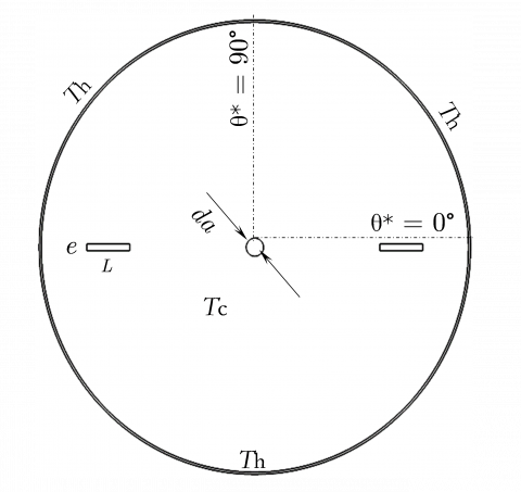
Figure 2 shows a cross section of this tank, which represents the computation domain. We note here that the longitudinal plane of equation θ* = 0 is that of the agitator and its extension towards the wall of the tank, and the plane of equation θ* = 90° is the median plane. The geometric parameters of the tank are characterized by the following ratios: d/D = 0.779, da/D = 0.025, L/d = 0.074, w/D = 0.02 and H = D.
Figure 1. Stirred tank geometry
Figure 2. Computation domain
The tank is filled with the non-Newtonian shear thinning nanofluid (Al2O3-water), where the anchor which rotates around its shaft, in the negative direction. The wall of the tank is kept at a hot temperature Th and the external borders of the anchor are thermally insulated. The initial temperature of the tank is cold Tc the properties of the basic fluid and nanoparticles are mentioned in the Table 1.
Table 1. Physical properties of the base fluid and nanoparticles
|
|
Density [kg/m3] |
Heat capacity [J/(kg.K)] |
Thermal conductivity [W/(m.K)] |
Dynamic viscosity [kg/(m.s)] |
|
Water |
998.2 |
4182 |
0.597 |
9.93 10-4 |
|
Alumina |
3880 |
773 |
36 |
/ |
3.1 Dimensional equations
The anchor is part of the agitation mobiles essentially generating a tangential flow, therefore the axial velocity are relatively low compared to the tangential one.
The study of the flow in the agitated tank is assumed to be two-dimensional because of the very small dependence of the velocity field and temperature on the vertical axis.
The flow of non-Newtonian nanofluid in this case is governed by the continuity, the momentum and energy equations.
In order to simplify the study, a list of hypotheses has been introduced; the nanofluid is considered to be a homogeneous and isotropic medium. The flow in the agitated tank is laminar; this is obtained by reducing the rotation speed of the anchor. The preceding equations are introduced into a Cartesian coordinate system. The physical parameters of the non-Newtonian nanofluid containing alumina nanoparticles (Al2O3) were introduced into the differential system governing the physical model by the correlations of the nanometric suspension cited in the literature. The equation system governing the flow of the nanofluid is as follows:
$\frac{\partial U}{\partial X}+\frac{\partial V}{\partial Y}=0$ (1)
$\begin{array}{l}
\rho_{\mathrm{nf}}\left(\frac{\partial U}{\partial t}+U \frac{\partial U}{\partial X}+V \frac{\partial U}{\partial Y}\right)=-\frac{\partial P}{\partial X}+\left(\frac{\partial \tau_{X X}}{\partial X}+\frac{\partial \tau_{X Y}}{\partial Y}\right) \\
\rho_{\mathrm{nf}}\left(\frac{\partial V}{\partial t}+U \frac{\partial V}{\partial X}+V \frac{\partial V}{\partial Y}\right)=-\frac{\partial P}{\partial Y}+\left(\frac{\partial \tau_{X Y}}{\partial X}+\frac{\partial \tau_{Y Y}}{\partial Y}\right)
\end{array}$ (2)
$\frac{\partial T}{\partial t}+U \frac{\partial T}{\partial X}+V \frac{\partial T}{\partial Y}=\alpha_{\mathrm{nf}}\left(\frac{\partial^{2} T}{\partial X^{2}}+\frac{\partial^{2} T}{\partial Y^{2}}\right)$ (3)
With αnf is the nanofluid thermal diffusivity, it is given by:
$\alpha_{\mathrm{nf}}=\frac{k_{\mathrm{nf}}}{\rho_{\mathrm{nf}} C p_{\mathrm{nf}}}$ (4)
The nanofluid density and the specific heat are given by:
$\rho_{\mathrm{nf}}=\varphi \rho_{\mathrm{p}}+(1-\varphi) \rho_{\mathrm{f}}$ (5)
$(\rho C p)_{\mathrm{nf}}=\varphi(\rho C p)_{\mathrm{f}}+(1-\varphi)(\rho C p)_{\mathrm{p}}$ (6)
With φ is the volume fraction of nanoparticles suspended in water. The effective thermal conductivity coefficient of the nanofluid can be approximated by the Maxwell model [25]. This formula is limited for nanoparticles of spherical shape.
$\frac{k_{\mathrm{nf}}}{k_{\mathrm{f}}}=\frac{k_{\mathrm{p}}+2 k_{\mathrm{f}}-2 \varphi\left(k_{\mathrm{f}}-k_{\mathrm{p}}\right)}{k_{\mathrm{p}}+2 k_{\mathrm{f}}+\varphi\left(k_{\mathrm{f}}-k_{\mathrm{p}}\right)}$ (7)
For a purely viscous non-Newtonian nanofluid which follows the Ostwald - De Waele model (i.e. the power law), the shear stress tensor is:
$\tau_{i j}=2 \mu_{\mathrm{nf}} D_{i j}=\mu_{\mathrm{nf}}\left(\frac{\partial U_{i}}{\partial X_{j}}+\frac{\partial U_{j}}{\partial X_{i}}\right)$ (8)
where, Dij denotes the shear rate tensor for the two-dimensional Cartesian coordinate. The nanofluid viscosity is given by Brinkman's formula [26] as follows:
$\mu_{\mathrm{nf}}=\mu_{\mathrm{f}}(1-\varphi)^{-2.5}$ (9)
$\mu_{\mathrm{f}}=M\left\{2\left[\left(\frac{\partial U}{\partial X}\right)^{2}+\left(\frac{\partial V}{\partial Y}\right)^{2}\right]+\left(\frac{\partial U}{\partial Y}+\frac{\partial V}{\partial X}\right)^{2}\right\}^{\frac{n-1}{2}}$ (10)
Ostwald's law of behavior characterizes two types of fluid, pseudoplastic fluids and dilatant fluids. Shear thinning fluids coincide with the range of the behavior index n < 1; they are characterized by an apparent viscosity which decreases with increasing shear rate. When n = 1 it is a Newtonian behavior.
The following relation gives the stream function.
$\frac{\partial \psi}{\partial X}=-V \text { and } \frac{\partial \psi}{\partial Y}=U$ (11)
The tangential and radial velocities of the flow within the agitated tank are calculated by the expressions:
$V_{\theta}=\frac{-U Y+V X}{r} \text { and } V_{r}=\frac{U X+V Y}{r}$ (12)
3.2 Dimensionless equations
To simplify the writing of the initial boundary conditions, we have chosen a rotating reference frame linked to the agitator fixed with respect to the tank which rotates at the same rotation speed but in the opposite direction, taking into account the centrifugal acceleration and of Coriolis [1].
The hydrodynamic study has been considered to be done in a stationary regime. While assuming that heat transfer begins in the tank as soon as the flow becomes stationary.
In order to solve Eqns. (1), (2) and (3) and to generalize this phenomenon, the dimensionless variables are:
$\begin{array}{l}
t^{*}=2 \pi N t, X^{*}=\frac{2 X}{D}, Y^{*}=\frac{2 Y}{D}, U^{*}=\frac{U}{\pi N D}, \\
V^{*}=\frac{V}{\pi N D}, P^{*}=\frac{P}{\rho(\pi N D)^{2}} \text { and } T^{*}=\frac{T-T_{c}}{T_{h}-T_{c}}
\end{array}$ (13)
By substituting in Eqns. (1), (2) and (3) we will have:
$\frac{\partial U^{*}}{\partial X^{*}}+\frac{\partial V^{*}}{\partial Y^{*}}=0$ (14)
$\begin{array}{r}
\frac{\partial U^{*}}{\partial t^{*}}+U^{*} \frac{\partial U^{*}}{\partial X^{*}}+V^{*} \frac{\partial U^{*}}{\partial Y^{*}}=-\frac{\partial P^{*}}{\partial X^{*}}+\frac{2}{\pi}\left(\frac{d}{D}\right)^{2} \frac{\rho_{\mathrm{f}}}{\rho_{\mathrm{nf}}} \frac{(2 \pi)^{n-1}}{(1-\varphi)^{2.5} \mathrm{Re}} \\
\times\left[2 \frac{\partial}{\partial X^{*}}\left(\frac{\mu_{\mathrm{f}}^{*}}{M} \frac{\partial U^{*}}{\partial X^{*}}\right)+\frac{\partial}{\partial Y^{*}}\left(\frac{\mu_{\mathrm{f}}^{*}}{M}\left(\frac{\partial U^{*}}{\partial Y^{*}}+\frac{\partial V^{*}}{\partial X^{*}}\right)\right)\right]
\end{array}$ (15a)
$\begin{aligned}
\frac{\partial V^{*}}{\partial t^{*}}+U^{*} & \frac{\partial V^{*}}{\partial X^{*}}+V^{*} \frac{\partial V^{*}}{\partial Y^{*}}=-\frac{\partial P^{*}}{\partial Y^{*}}+\frac{2}{\pi}\left(\frac{d}{D}\right)^{2} \frac{\rho_{\mathrm{f}}}{\rho_{\mathrm{nf}}} \frac{(2 \pi)^{n-1}}{(1-\varphi)^{2.5} \mathrm{Re}} \\
& \times\left[2 \frac{\partial}{\partial Y^{*}}\left(\frac{\mu_{\mathrm{f}}^{*}}{M} \frac{\partial V^{*}}{\partial Y^{*}}\right)+\frac{\partial}{\partial X^{*}}\left(\frac{\mu_{\mathrm{f}}^{*}}{M}\left(\frac{\partial U^{*}}{\partial Y^{*}}+\frac{\partial V^{*}}{\partial X^{*}}\right)\right)\right]
\end{aligned}$ (15b)
$\frac{\partial T^{*}}{\partial t^{*}}+U^{*} \frac{\partial T^{*}}{\partial X^{*}}+V^{*} \frac{\partial T^{*}}{\partial Y^{*}}=\frac{2 \alpha_{\mathrm{nf}}\left(\frac{d}{D}\right)^{2}}{\pi \alpha_{\mathrm{f}} \mathrm{Re} \operatorname{Pr}}\left(\frac{\partial^{2} T^{*}}{\partial X^{* 2}}+\frac{\partial^{2} T^{*}}{\partial Y^{* 2}}\right)$ (16)
The dimensionless stream function is given by:
$\frac{\partial \psi^{*}}{\partial X^{*}}=-V^{*} \text { and } \frac{\partial \psi^{*}}{\partial Y^{*}}=U^{*}$ (17)
The dimensionless initial boundaries conditions are:
$\text { Tank wall : } r^{*}=1: V_{\theta \text { fixed }}^{*}=-1 \text { and } V_{r}^{*}=0$ (18a)
$\text { Anchor boundaries: } V_{\theta \text { fixed }}=V_{r}=0$ (18b)
At the initial time t* = 0
$\text { Tank wall: } T^{*}=1$ (18c)
$\text { The entire tank: } T^{*}=0$ (18d)
$\text { Anchor boundaries: } \partial_{n} T^{*}=0$ (18e)
The dimensionless numbers that appear in the dimensionless Eqns. (14)-(16) are the Reynolds number characterizing the phenomenon of inertia, the Prandtl number and the dimensionless viscosity.
$\mathrm{Re}=\frac{\rho_{\mathrm{f}} N^{2-n} d^{2}}{M}$ (19)
$\operatorname{Pr}=\frac{M C p_{\mathrm{f}} N^{n-1}}{k_{\mathrm{f}}}$ (20)
$\mu_{\mathrm{f}}^{*}=\frac{\mu_{\mathrm{f}}}{(2 \pi N)^{n-1}}$ (21)
The Reynolds number which governs the laminar flow of the viscous flow without taking into account the influence of the concentration of nanoparticles is given by the following relation:
$\mathrm{Re}_{\mathrm{nf}}=\frac{\mu_{\mathrm{f}}}{\mu_{\mathrm{nf}}} \frac{\rho_{\mathrm{nf}} N^{2-n} d^{2}}{M}$ (22)
The Eq. (22) allows us to deduce the relation:
$\mathrm{Re}_{\mathrm{nf}}=\frac{\mu_{\mathrm{f}}}{\mu_{\mathrm{nf}}} \frac{\rho_{\mathrm{nf}}}{\rho_{\mathrm{f}}} \frac{\rho_{\mathrm{f}} N^{2-n} d^{2}}{M}$ (23)
We therefore define the dimensionless Reynolds number as:
$\mathrm{Re}^{*}=\frac{\operatorname{Re}_{\mathrm{nf}}}{\operatorname{Re}}=(1-\varphi)^{2.5}\left[\varphi \frac{\rho_{\mathrm{p}}-\rho_{\mathrm{f}}}{\rho_{\mathrm{f}}}+1\right]$ (24)
The number Re* varies as a function of φ. The derivative of Re* from expression Eq. (24) give:
$\frac{\mathrm{d} \mathrm{Re}^{*}}{\mathrm{~d} \varphi}=(1-\varphi)^{1.5}\left[\frac{\rho_{\mathrm{p}}-\rho_{\mathrm{f}}}{\rho_{\mathrm{f}}}(1-3.5 \varphi)-2.5\right]$ (25)
The maximum value of Re* is determined by canceling the derivative of Re* Eq. (25) which gives:
$\varphi_{0}=\frac{2 \rho_{\mathrm{p}}-7 \rho_{\mathrm{f}}}{7\left(\rho_{\mathrm{p}}-\rho_{\mathrm{f}}\right)} \simeq 0.038$ (26)
Power number: It is a dimensionless parameter that provides a measure of the power requirements for the operation of an impeller. It is defined as:
$\mathrm{Np}=\frac{\mathrm{P}}{\rho N^{3} d^{5}}$ (27)
With P is the power consumed which, according to reference [2] is equal to the following expression:
$\mathrm{P}=\int_{\text {Tnak volume }} \mu_{\mathrm{nf}} Q_{V} \mathrm{~d} W$ (28)
In dimensionless terms, the power number is given by:
$\mathrm{Np}=\frac{H}{8}\left(\frac{D}{d}\right)^{3} \frac{(2 \pi)^{n+1}}{\mathrm{Re}} \iiint_{\text {Trak volume }} \mu_{\mathrm{f}}^{*} Q_{V}^{*} \mathrm{~d} X^{*} \mathrm{~d} Y^{*}$ (29)
With $Q_{V}^{*}$ is the dimensionless viscous dissipation.
$Q_{V}^{*}=2\left[\left(\frac{\partial U^{*}}{\partial X^{*}}\right)^{2}+\left(\frac{\partial V^{*}}{\partial Y^{*}}\right)^{2}\right]+\left(\frac{\partial U^{*}}{\partial Y^{*}}+\frac{\partial V^{*}}{\partial X^{*}}\right)^{2}$ (30)
Modified power number: To visualize the influence of viscosity on the variation of the stirring power, just divide Eq. (29) by ρfN3d5 instead of ρnfN3d5.
$\mathrm{Np}_{\mathrm{mod}}=\frac{\rho_{\mathrm{nf}}}{\rho_{\mathrm{f}}} \mathrm{Np}$ (31)
Nusselt number: Which characterizes forced convection in the entire tank, it is defined as:
$\mathrm{Nu}_{r}=\frac{k_{\mathrm{nf}}}{k_{\mathrm{f}}}\left(\frac{\partial T^{*}}{\partial X^{*}} \cos \theta+\frac{\partial T^{*}}{\partial Y^{*}} \sin \theta\right)$ (32)
The average instantaneous Nusselt number is calculated by the average of the local Nusselt number on the hot wall (which is here the wall of the tank).
$\mathrm{Nu}=\frac{1}{\pi D_{\text {Tank wall }}} \oint \mathrm{Nu}_{D / 2} \mathrm{~d} \theta$ (33)
Figure 3. Computation domain mesh
The system of Eqns. (14)-(16), provided with the boundary conditions Eqns. (18a)-(18e) is solved by the finite element method based on Galerkin's discretization. The adopted mesh of the computation domain is triangular and refined near the anchor walls as shown in Figure 3. An adequate number of elements was tested so as to obtain results very close to those existing in the literature. The chosen convergence criterion is linked to the relative error of variables less than 10-6.
To be able to make our numerical study of the incompressible flow of a shear thinning nanofluid, we compared our numerical results with those of the literature.
(a) Tangential velocity
(b) Power number
Figure 4. Results comparaison
Figure 4 shows the variation of the tangential velocity on the agitator plane and its extension to the wall of the tank (Figure 4a), and the variation of the power number as a function of the Reynolds number (Figure 4b), for the present work and for references [1, 5]. The comparison of the results shows a good agreement.
5.1 Hydrodynamic results
5.1.1 Effect of inertia
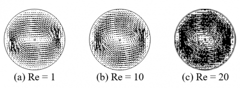
Figure 5 presents the flow velocity field of a nanofluid with a concentration of 0.04 and a pseudoplastic behavior index of 0.7 for three different Reynolds numbers (1, 10 and 20). We see that the tangential flow is dominant in the tank with an intensity translated by the importance of the velocity field at the level of anchor blades. There is a certain symmetry of the velocity field with respect to the mediator line for the low Reynolds number (Re = 1). This symmetry is lost for the highest Reynolds numbers (Re = 10 and 20) which clearly shows the radial displacement of the flow. Between the blade and the inner wall of the tank there is a slowing of the flow favoring the creation of the two-recirculation loops, which lose their existence as the Reynolds number increases.
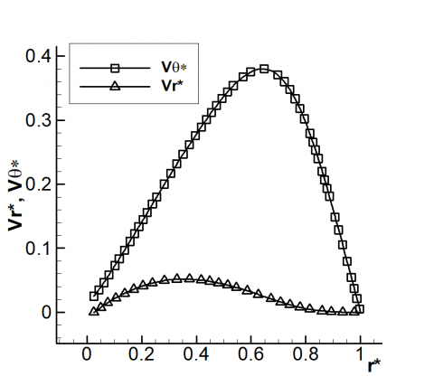
Figure 6 presents the tangential and radial velocity in the same frame on the anchor plane and its extension to the tank wall and on the median plane, for the nanofluid of φ = 0.04, n = 0.7 and Re = 20. The first observation that can be made is the dominance of the tangential velocity on the two measurement planes, where the radial velocity exhibits relatively weak behavior on the median plane. On the agitator plane (Figure 6a), the tangential velocity increases from the anchor shaft to the end of the blade, while satisfying linear growth along the blade until an extreme value (d/D), this velocity decreases from the end of the blade until it vanishes on the outer tank wall. The radial velocity presents a behavior different from that of the tangential velocity, where it increases while going inward then it decreases abruptly in the immediate vicinity of the blade. Along the blade, the radial velocity is completely zero by designating that the flow is purely tangential with this blade, downstream of the blade, there is a sudden increase in the direction of the wall, which favors the radial flow, and it loses its intensity in the immediate vicinity of the internal tank wall. Along the perpendicular bisector (Figure 6b), the tangential velocity increases faster than that of the blade to reach a maximum near 0.38 at r* = 0.62 then it begins to decrease rapidly to cancel out at the wall. The radial velocity increases slightly in a concave manner in the direction of outside flow, then it presents a slow convex decrease to cancel out on the wall.
Figure 5. Velocity field within the agitated tank
(a) Agitator plane
(b) Median plane
Figure 6. Tangential and radial velocity
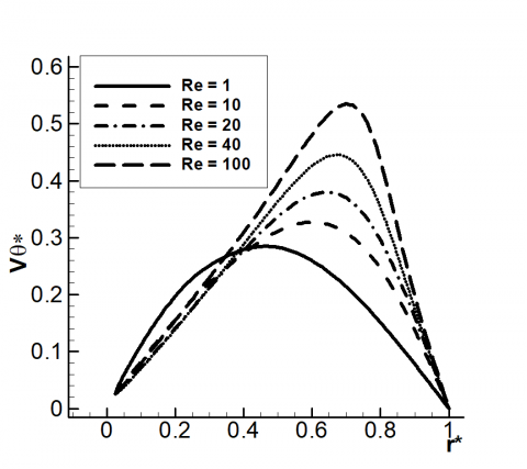
Figure 7 illustrate the influence of Re on the tangential velocity on the two measurement planes, with a nanofluid having φ = 0.04 and n = 0.7. The inertia influences positively on the tangential velocity at the agitator plane, where this velocity increases as a function of Re, the rate of increase of this velocity becomes more important for the transition Reynolds numbers (concavity of the curves).
(a) Agitator plane
(b) Median plane
Figure 7. Tangential velocity for different Re
On the anchor blade (Figure 7a), the variation of the tangential velocity is identical. For a low Reynolds number downstream of the blade, a change in sign of the tangential velocity has been noted, which indicates the existence of recirculation loops. This negative sign no longer exists for the greatest Re numbers, which leads to the disappearance of its zones. On the median plane (Figure 7b), the inertia decreases the tangential velocity next to the shaft then it increases it.
The widening of the suction zone, located upstream of two anchor blades causes this hydrodynamics.
5.1.2 Effect of volume fraction
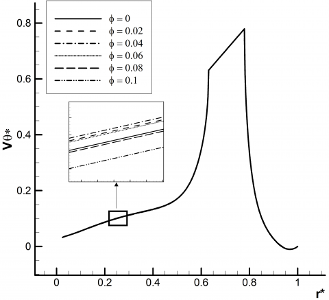
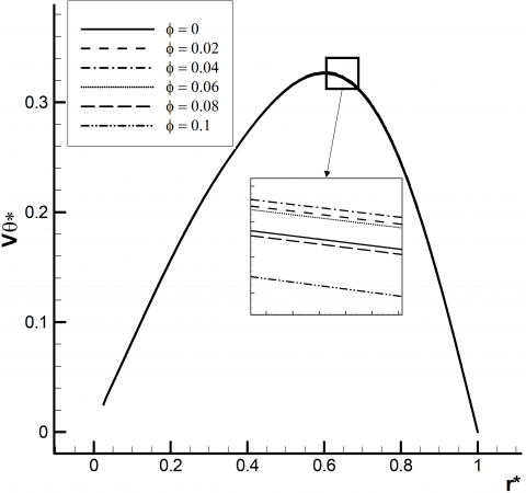
Figures 8 and 9 illustrate the distribution of the tangential velocity on the two measurement planes for different nanoparticles volume fraction for n = 0.7 and Re = 10.
Figure 8. Tangential velocity on agitator plane for different φ
Figure 9. Tangential velocity on median plane for different φ
It can be seen in these figures that the influence of alumina concentration is very small, this comes down to three important causes: the nanometric size of the alumina particles, their low mass and the low concentrations used in the simulation. After zooming in on certain zones, we have observed the existence of two intervals of volume fraction influence on the tangential velocity: the concentrations below φ0 (Eq. (26)) and those above this concentration. Along the extension of the blade (Figure 8) the tangential velocity increases for φ < φ0 while it decreases for φ > φ0. On the perpendicular bisector (median plane), there are two zones like those of Reynolds number (Figure 7), where the nanoparticle concentration keeps the same impact as that of the agitator plane. The effects of the kinematic viscosity can interpret the variable effect of the volume fraction on the velocity profile. In fact, the introduced of the fraction volume of nanoparticle into the momentum equations causes a rise in density and dynamic viscosity according to Brinkman's law [26]; this increase on proprieties leads also to a non-monotonic variation of the kinematic viscosity.
5.1.3 Effect of behavior index
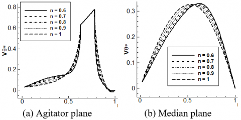
Figure 10 presents the distribution of the tangential velocity, on the agitator extension plane and on the median plane for different behavior index (n = 0.6 to 1). The nanofluid have a concentration of 0.04 and Re = 10. On the of the agitator plane between the shaft and the blade, the shear thinning behavior leads to an increase in tangential velocity in the area close to the center of the tank as well as its internal wall, there is an inverse effect in the vicinity of the blade and in the immediate vicinity downstream thereof. This is due to the importance of the apparent viscosity of the nanofluid, which increases by the effect of slow variations in the shear rate around the shaft and in the immediate vicinity of the internal wall of the tank. On the anchor plane there is an increase in the tangential velocity with the decrease in the behavior index and then an increase.
Figure 10. Tangential velocity for different n
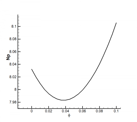
5.2 Power consumption
Figure 11 illustrates the variation of the power number as a function of the alumina volume fraction. The power number decreases slightly to a minimum corresponding to the concentration φ0. Beyond this concentration, there is an increase in the power number. In reality, the high power consumed depends on the increase in the nanoparticles fraction, which amounts to a relative increase in the dynamic viscosity of the nanofluids compared to their base fluid. Obtaining the power number comes down to dividing the power P, which varies with the apparent viscosity of the fluid and the viscous dissipation Eq. (28) by the term ρnfN3d5. The modification consists in dividing the power by ρfN3d5, which shows us exactly the consumption of the power.
Figure 11. Power number as function of φ
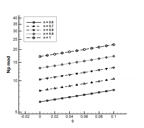
Figures 12 and 13 show the variation of the modified power number depending on the alumina fraction for different Re (Figure 12) and for different behavior index (Figure 13). The power number increases always with the rise of volume fraction for all Reynolds numbers and all behavior index. In the other hand, we noted an increase in power number when the behavior index falls, as well as a decrease when the Reynolds number rises. This reduction comes back to the pseudoplastic behavior presented by the mixture Al2O3-water which provokes a decrease in apparent dynamic viscosity when the shear rate augments.
Figure 12. Modified power number as function of φ
Figure 13. Modified power number as function of φ for different n
Therefore, an optimal power consumption for the rise nanoparticles volume fractions has been verified when the shear-thinning index falls, with mean Reynolds numbers.
5.3 Thermal results
In this part we give our results at the dimensionless instant t* = 8 and Pr = 7. In the Figures 14, 15 and 16 we give streamlines (right column) and isotherms (right column).
In Figure 14, a pattern of streamlines and isotherms are shown, at the cross section of the stirred tank. The nanofluid has a concentration of 0.04 and a behavior index of 0.7, for the Reynolds numbers zone take almost the same streamlines shape for Re equals to 10 and 20. Far from the center of the tank, the streamlines and the isotherms are substantially parallel to the tank wall. The temperature rises rapidly (from the hot wall) of (1, 10 and 20) at time t*= 8.
It is clear that the structure is practically symmetrical with respect to the center of the tank regardless of the Re number. A rotating movement in block of the nanofluid with the agitator characterizes the zone close to the agitator shaft, where the streamlines are closed curves; this means the existence of a vortex. The isotherms in this throughout the tank for the low Reynolds numbers. Moreover, we find that the important temperature gradients correspond to the greatest Reynolds numbers. For Re = 1 the process of the conductive heat transfer is the most dominant, where we marked a nonconformity between the streamlines and the isotherms.
Figure 14. Streamlines and isotherms for different Re
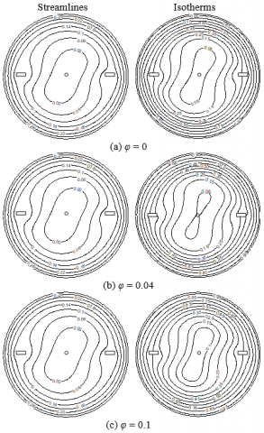
Figure 15, presents the streamlines and the isotherms in the whole of the tank with Al2O3-water, for behavior index of 0.7 and Re = 10 and for different volume fractions of nanoparticles (0, 0.04 and 0.1). We have noted an identification of streamlines for all volume fraction, which comes down essentially to the very small variations of the velocity field in the tank. In the order hand, there is an acceleration of the heat flux for the volume fractions 0.04 and 0.1. Moreover, the tendency of the isotherms toward moving to the anchor shaft increase noticeably compared to basic fluid, where we have noted the disappearance of the isotherm carrying the value 0.05 for the alumina concentration of 0.1 and the other contours became narrow.
A decrease in the unsteady thermal gradient in the tank has been observed for the largest volume fractions indicating the decrease in the thermal stability time. As for the streamlines, there is a consistency between the nanofluid streamlines and the isotherms pattern for all volume fractions. The comparison between isotherms of the nanofluid and the base fluid exhibits that the rate of heat transfer augments with the addition of the nanoparticles.
Figure 15. Streamlines and isotherms for diferent φ
Figure 16 shows a pattern of streamlines and isotherms for a nanofluid having φ = 0.04, Re = 10 and for different behavior index (0.6, 0.8 and 1). Analysis of these contours shows a small variation in the patterns of flow currents and temperature profile. There is an expansion of the streamlines in the direction of the median plane and a slight contraction in width on the extension of agitator plane. The isotherms follow the same patterns as those of the streamlines. It is noted that a small decrease in temperature value has been observed as the shear tinning behavior augments. Moreover, the nanofluid isotherms heads towards the hot wall more than the anchor shaft, comparing with the Newtonian case (n = 1). Therefore, it confirms that the heat transfer declines weakly with the drop of the flow behavior index.
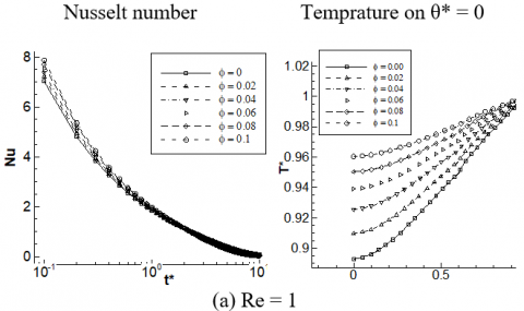
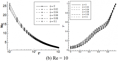
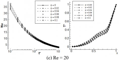
Figure 17 illustrates the variation of the instantaneous average Nusselt number as a function of dimensionless time and (the left column) and the variation of the temperature on the agitator plane and its extension (right column) for different volume fractions and different Reynolds numbers. Whatever the Reynolds number and the volume fraction, the instantaneous average Nusselt number decreases as a function of time until it vanishes at the end of the heat transfer (the instant of stability). This low Nusselt number indicates that the heat transfer drops over time, reason that the temperature gradient decreases as a function of time. An enhancement in the heat transfer has been demonstrated with the improvement in the volume fraction of alumina in the water regardless of the Re number. However, the rate of heat transfer enhancement decreases as a function of time until it vanishes beyond moments of thermal stability.
Figure 16. Streamlines and isotherms for diferent n
In the other hand, the Nusselt number also augments with the rise Reynolds number for all volume fractions. Regarding dimensionless temperature, it increases on the plane of the agitator and its extension, up to the value of stability. There is a quasi-linear temperature rise on the anchor blade, which characterized by a decrease in temperature gradients due to the tangential flow intensity near the blade. Moreover, the highest temperatures have been observed for the highest alumina volume fractions. It is worth noting here, the low Reynolds numbers leads to arise in temperature value with low thermal gradients.
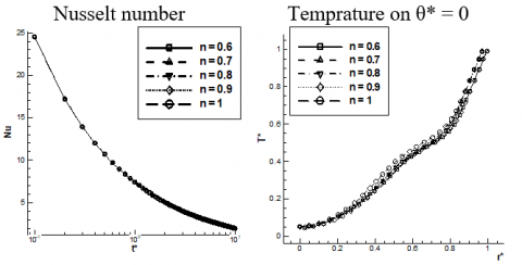
Figure 18 presents the variation of the instantaneous Nusselt number for different behavior index. The influence of this index on the Nusselt number was not visible, quite for the isotherms and the current lines. However, through the streamlines (Figure 14), we were able to know that the temperature resulted in a very slight reduction in heat transfer. In other way, the variation of the temperature on the extension of the agitator follows the same pattern as that of the volume fraction (Figure 15), where the maximum temperature is corresponding to the behavior index n = 1 (Newtonian) and falls by decreasing this index. The same process would have been noted if the Reynolds number had been changed.
Figure 17. Average Nusselt number and temperature distribution for different Re and φ
Figure 18. Average Nusselt number and temperature distribution for different n
Table 2 shows the values of average instantaneous Nusselt number at the dimensionless time t* = 0.1, for different volume fractions and different Reynolds number. The table shows an enhancement in heat transfer in the region of 12% for the volume fraction of 0.1. There is also a small increase in the Nusselt improvement rate as a function of the number of Re. here we have chosen a primary instant given the clarity of the difference between the Nusselt numbers in these instant. A reduction in the improvement as a function of time has also been observed from the curves of Figure 15.
Table 2. Nusselt number and its improvement rate for different fraction and Re number
|
t* = 0.1 |
Re = 1 |
Re = 20 |
||
|
|
Nu |
ΔNu/Nuf |
Nu |
ΔNu/Nuf |
|
φ = 0 |
7.04 |
|
33.24 |
|
|
φ = 0.02 |
7.20 |
2.27% |
34.08 |
2.52% |
|
φ = 0.04 |
7.37 |
4.68% |
34.92 |
5.05% |
|
φ = 0.06 |
7.53 |
6.96% |
35.77 |
7.61% |
|
φ = 0.8 |
7.69 |
9.23% |
36.61 |
10.13% |
|
φ = 0.1 |
7.86 |
11.64% |
37.55 |
12.96% |
In this study, thermal and hydrodynamic effect of a non-isothermal laminar flow in an agitated tank equipped with an anchor, filled with Al2O3-water nanofluid while the mixture presents a shear thinning behavior has been analyzed by finite element method. The influence of different volume fraction, Reynolds number and shear thinning behavior index has been highlighted. This study demonstrates an improvement in heat transfer with the increase in the nanoparticles volume fraction where the highest Nusselt number was obtained in 10% volume fraction Al2O3-water nanofluid, as well as a small decrease in this transfer with the important shear thinning behavior index. It was also found that the major influence of alumina nanoparticles on the enhancement of heat transfer has been verified for high Reynolds numbers. However, we noted a relatively small increase in power number for the high concentration of nanoparticles indicating that the energy consumption increase; on the other hand, we noted better energy consumption for nanofluids with the lowest behavior index. In terms of optimization, the best heat transfer while maintaining good energy consumption corresponds to the nanofluid having a high fraction and a low behavior index. To give an additional dimension to this work, we recommend focusing on the study of the nanofluids flow by taking into account the effect of Brownian motion and thermophores on this flow.
|
t |
Time [s] |
|
X, Y |
Cartesian coordinates [m] |
|
U |
Velocity in X direction [m.s-1] |
|
V |
Velocity in Y direction [m.s-1] |
|
P |
Pressure [Pa] |
|
T |
Temperature [K] |
|
r |
Radial coordinate [m] |
|
D |
Tank diameter [m] |
|
d |
Agitator diameter [m] |
|
L |
Blade length [m] |
|
da |
Shaft diameter [m] |
|
w |
Blade width [m] |
|
H |
Tank hauteur [m] |
|
Cp |
Specific heat [J.kg-1.K-1] |
|
M |
Consistency coefficient [kg.(m.s2 – n)-1] |
|
n |
Flow index behavior |
|
k |
Thermal conductivity [W.m-1.K-1] |
|
N |
Rotation speed [s-1] |
|
Re |
Reynolds number |
|
Pr |
Prandtl number |
|
Nu |
Nusselt number |
|
Np |
Power number |
|
Greek symbols |
|
|
ρ |
Density [kg.m-3] |
|
μ |
Dynamic viscosity [kg.m-1 s-1] |
|
φ |
Volume fraction |
|
τ |
Shear stress [pa] |
|
ψ |
Stream function |
|
θ |
Tangential coordinate [rd] |
|
Subscripts |
|
|
p |
Nanoparticules |
|
f |
Basic fluid |
|
nf |
Nanofluid |
[1] Bertrand, J. (1983). Agitation des fluids visqueux cas de mobiles à pales, d’ancre et de barrières. Thèse de doctorat, Istitut nationale polytechnique de Toulouse.
[2] Bertrand, J., Couderc, J.P. (2009). Agitation de fluides pseudoplastiques par un agitateur bipale. The Canadian Journal of Chemical Engineering, 60(6): 738-747. https://doi.org/10.1002/cjce.5450600604
[3] Bertrand, J., Abid, M., Xuerb, C. (1992). Hydrodynamics in vessels stirred with anchors and gate agitators: Necessity of 3-D modelling. Chemical Engineering Research and Design, 70: 377-384.
[4] Baccar, M., Mseddi, M., Abid, M.S. (2001). Contribution numérique à l’étude hydrodynamique et thermique des écoulements turbulents induits par une turbine radiale en cuve agitée. Int. J. Therm. Sci, 40(8): 753-772. https://doi.org/10.1016/S1290-0729(01)01263-7
[5] Hami, O., Draoui, B., Mebarki, B., Rahmani, L., Bouanini, M. (2008). Numerical model for laminar flow and heat transfer in an Agitated vessel by inclined blades anchor. Proceedings of CHT-08 ICHMT International Symposium on Advances in Computational Heat Transfer. Marrakech, Morocco. https://doi.org/10.1615/ICHMT.2008.CHT.1270
[6] Rahmani, L., Mebarki, B. Allaoua, B., Draoui, B. (2013). Laminar flow characterization in a stirred tank with a gate impeller in case of a non-Newtonian fluid. Energy Procedia, 36: 418-427. https://doi.org/10.1016/j.egypro.2013.07.048
[7] Benmoussa, A., Rahmani, L. (2018). Numerical analysis of thermal behavior in agitated vessel with non-Newtonian fluid. Int. Jnl. of Multiphysics, 12(3): 209-220. https://doi.org/10.21152/1750-9548.12.3.209
[8] Ameur, H., Bouzit, M., Helmaoui, M. (2012). Hydrodynamic study involving a Maxblend impeller with yield stress fluids. Journal of Mechanical Science and Technology, 26(5): 1523-1530. https://doi.org/10.1007/s12206-012-0337-3
[9] Ameur, H. (2016). Effect of some parameters on the performance of anchor impellers for stirring shear-thinning fluids in a cylindrical vessel. Journal of Hydrodynamics, 28(4): 669-675. https://doi.org/10.1016/S1001-6058(16)60671-6
[10] Choi, S.U.S., Eastman, J.A. (1995). Enhancing thermal conductivity of fluids with nanoparticles. 1995 International mechanical engineering congress and exhibition, San Francisco, CA (United States), pp. 99-105.
[11] Pak, B.C., Cho Y.I. (1998). Hydrodynamic and heat transfer study of dispersed fluids with submicron metallic oxide particles, experimental heat transfer. A Journal of Thermal Energy Generation, Transport, Storage, and Conversion, 11(2): 151-170. https://doi.org/10.1080/08916159808946559
[12] Eastman, J.A., Phillpot, S.R, Choi, S.U.S., Keblinski, P. (2004). Thermal transport in nanofluids. Annu. Rev. Mater. Res, 34(1): 219-246. https://doi.org/10.1146/annurev.matsci.34.052803.090621
[13] Patel, H.E., Das, S.K., Sundararajan, T. (2003). Thermal conductivities of naked and monolayer protected metal nanoparticle based nanofluids: Manifestation of anomalous enhancement and chemical effects. Appl. Phys. Lett, 83(14): 2931-2933. https://doi.org/10.1063/1.1602578
[14] Abu-Nada, E., Masoud, Z., Oztop, H.F., Campo, A. (2010). Effect of nanofluid variable properties on natural convection in enclosures. Int. J. Therm. Sci, 49(3): 479-491. https://doi.org/10.1016/j.ijthermalsci.2009.09.002
[15] Perarasu, V.T., Arivazhagan M., Sivashanmugam, P. (2012). Heat transfer of TiO2/water nanofluid in a coiled agitated vessel with propeller. Journal of Hydrodynamics, 24(6): 942-950. https://doi.org/10.1016/S1001-6058(11)60322-3
[16] Perarasu, T., Arivazhagan, M., Sivashanmugam, P. (2013). Experimental and CFD heat transfer studies of Al2O3-water nanofluid in a coiled agitated vessel equipped with propeller. Chinese Journal of Chemical Engineering, 21(11): 1232-1243. https://doi.org/10.1016/S1004-9541(13)60579-0
[17] Srinivas, T., Vinod, A.V. (2013). Performance of an agitated helical coil heat exchanger using Al2O3/water Nanofluid. Experimental Thermal and Fluid Science, 51: 77-83. http://doi.org/10.1016/j.expthermflusci.2013.07.003
[18] Naik, B.A.K., Vinod, A.V. (2018). Heat transfer enhancement using non-Newtonian nanofluids in a shell and helical coil heat exchanger. Experimental Thermal and Fluid Science, 90: 132-142. https://doi.org/10.1016/j.expthermflusci.2017.09.013
[19] Alami, A.H., Abu Hawili, A., Aokal, K., Faraj, M., Tawalbeh, M. (2020). Enhanced heat transfer in agitated vessels by alternating magnetic field stirring of aqueous Fe–Cu nanofluid. Case Studies in Thermal Engineering 20: 100640. https://doi.org/10.1016/j.csite.2020.100640
[20] Srinivas, T., Venu Vinod, A. (2016). Heat transfer intensification in a shell and helical coil heat exchanger using water-based nanofluids. Chemical Engineering and Processing: Process Intensification, 102: 1-8. https://doi.org/10.1016/j.cep.2016.01.005
[21] Sajadifar, S.A., Karimipour, A., Toghraie, D. (2016). Fluid flow and heat transfer of non-Newtonian nanofluid in a microtube considering slip velocity and temperature jump boundary conditions. European Journal of Mechanics B/Fluids. http://dx.doi.org/10.1016/j.euromechflu.2016.09.014
[22] Hassani, M., Lavasani M.A., Kim, Y.S., Ghergherehchi, M. (2019). Numerical investigation of nanofluid Al2O3/water in elliptical tube equipped with twisted tape. International Journal of Heat and Technology, 37(2): 520-526. https://doi.org/10.18280/ijht.370219
[23] Mondal, M., Biswas, R., Shanchia, K., Hasan, M., Ahmmed, S.F. (2019). Numerical investigation with stability convergence analysis of chemically hydromagnetic Casson nanofluid flow in the effects of thermophoresis and Brownian motion. International Journal of Heat and Technology, 37(1): 59-70. https://doi.org/10.18280/ijht.370107
[24] Muthya Gouda, V., Vaisakhb, V., Josephb, M., Sajithb, V. (2020) An experimental investigation on the evaporation of polystyrene encapsulated phase change composite material based nanofluids. Applied Thermal Engineering, 168114862. https://doi.org/10.1016/j.applthermaleng.2019.11486
[25] Maxwell, J.C. (1881). A Treatise on Electricity and Magnetism, vol. II, Oxford University Press, Cambridge, UK, 1873. p. 54.
[26] Brinkman, H.C. (1952). The viscosity of concentrated suspensions and solutions. J. Chem. Phys, 20: 571-581. https://doi.org/10.1063/1.1700493