OPEN ACCESS
Autogyros are important for their maneuverability and operative flexibility. This paper defines a new autogyro configuration based on cyclorotors placed on the side of the cabin, near the centre of gravity of the aircraft, and a pushing propeller with horizontal axis. The used cyclorotor has an innovative high lift-resistive configuration that can maximize vertical lift, vertical propulsion and energy harvesting. The resulting aircraft has really breakthrough features. It can produce different configurations such as VTOL operation by using the cyclorotors for propulsion by mean electric motors, cogeneration during flight because of the autorotation of the cyclorotors and onboard energy harvesting by the reciprocal use of the motors as generators, fixed wing flight such as an old multi-wing aircraft of the pioneering era of aeronautics. The preliminary design process by the fundamental laws of basic physics is presented. An effective optimization of energetic equation of the resulting aircraft has been produced according to a second principle analysis of a theoretical model of the aircraft. The adopted method has been EMIPS that considers the resources required to move vehicle and payload to focus the analysis on the energetic inefficiencies at vehicle level.
autogyro, energy, exergy evaluation, electric cogeneration, EMIPS
A gyroplane or autogyro is an aircraft that is propelled by an engine driven propeller and produces the necessary lift by turning rotary wing [1]. It obtains remarkably high lift forces from a system of freely rotating blades that is actuated in similar way with respect to wind turbine. It has been intend by La Cierva [2], which has been presented for the first time in 1923. Its behaviour can be described by the simplified model by Glauert [3]. Glauert model is mostly phenomenological, and not mathematically well founded.
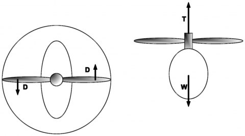
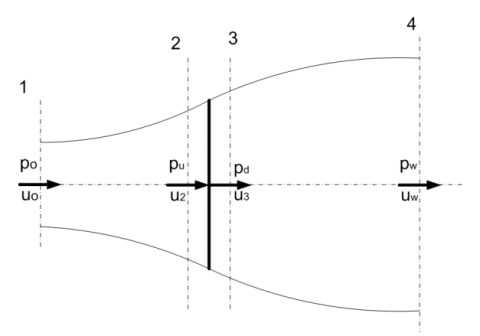
Figure 1. Simplified model of an autogyro
Otherwise, it gives reasonable estimates of inflow velocity at the rotor disk and gives the correct results for an elliptically loaded wing (Figure 1).
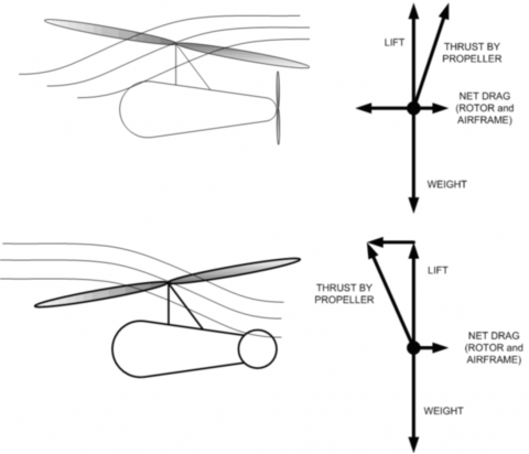
Figure 2. Preliminary conceptual representation of an autogyro during motion and comparison with helicopter
The compared models of flight of a helicopter and an autogyro are presented by Leishman [1] and are summarized in Figure 2.
1.1 Equation of the vehicle
Zuang et al [4] has defined a well working mathematical model of helicopter based on energy equations. They have described the energy behaviour of a helicopter in flight on a vertical plane by using the following equation:
$E=\frac{1}{2}\cdot m\cdot {{u}^{2}}+m\cdot g\cdot h+\frac{1}{2}\cdot I\cdot {{\Omega }^{2}}$ (1)
The term 0.5 I Ω2 can be assumed constant (and its derivative almost null in comparison with the other terms) because of the angular velocity Ω is almost constant and the inertia of the rotor I is lower with respect to the mass of the aircraft. Equation (1) can be expressed with respect to the direction of velocity with respect to x and y directions.
$E=\frac{1}{2}\cdot m\cdot \left( u_{x}^{2}+u_{y}^{2} \right)+m\cdot g\cdot h+\frac{1}{2}\cdot I\cdot {{\Omega }^{2}}$ (2)
The partial derivative with respect to time of equation (2) allows expressing the energy rate.
$\frac{dE}{dt}=P=m\cdot \left( {{u}_{x}}\frac{d{{u}_{x}}}{dt}+{{u}_{y}}\cdot \frac{d{{u}_{y}}}{dt} \right)+m\cdot g\cdot {{u}_{y}}$ (3)
A similar equation can be used also for modelling the energy behaviour of autogyros.
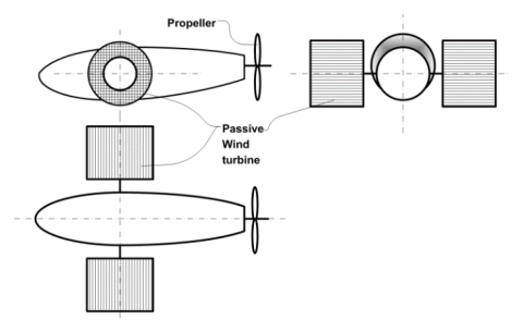
Figure 3. Preliminary layout of the new vehicle
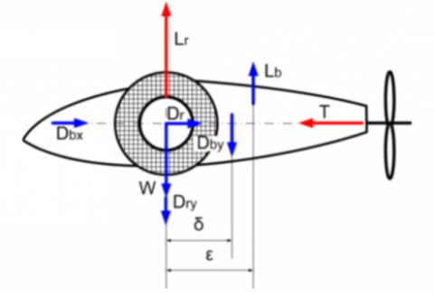
Figure 4. Forces applied on the vehicle
This paper considers the hypothesis of a new autogyro based on two rotating cylindrical wind turbines placed on the sides of the fuselage (Figure 3).
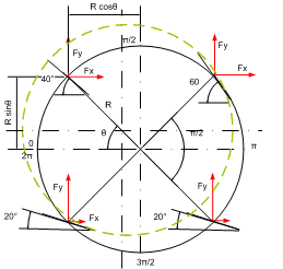
Forces acting on the vehicle are represented in figure 4.
The equilibrium of the forces gives the following system:
$\left\{\begin{array}{l}{M a_{x}=\Sigma_{i} F x} \\ {M a_{y}=\Sigma_{i} F_{y}} \\ {I \dot{\omega}_{z}=\Sigma_{i} M_{z}} \\ {0=\Sigma_{i} M_{y}}\end{array} \Rightarrow\left\{\begin{array}{l}{M a_{x}=T-D_{b x}+D_{r x}} \\ {M a_{y}=L_{r}+L_{b}-W-D_{r y}-D_{b y}} \\ {I \dot{\omega}_{z}=\varepsilon \cdot L_{b}+\delta \cdot D_{b y}} \\ {M_{p}+M_{r}=0}\end{array}\right.\right.$ (4)
1.2 Equations of the wind turbine
A simple model, attributed to Betz, [5] can be used to determine the power, the thrust of the wind on the ideal rotor and the effect of the rotor operation on the local wind field. By actuator disk simplification, the following assumptions can be made:
Figure 5. Actuator disk model
From the assumption that the continuity of velocity through the disk exists, the velocities at section 2 and 3 are equal to the velocity at the rotor
${{u}_{2}}={{u}_{3}}={{u}_{R}}$
and for steady flow, the mass flow rate through the disk is:
$\dot{m}=\rho \cdot A\cdot {{u}_{R}}$ (5)
The law of conservation of linear momentum applied to the control volume that encloses the system allows determining the net force produced by impinging air:
$F=\dot{m}\cdot ({{u}_{o}}-{{u}_{w}})=-T$ (6)
that is equal and opposite to the thrust T that wind applies on the wind turbine.
Considering the difference of pressure through the actuator disk it can be expressed the force (or thrust) as a function of the difference of pressure through the disk
$F=\dot{m}\cdot ({{u}_{o}}-{{u}_{w}})=-T=\Delta p\cdot {{A}_{d}}=({{p}_{u}}-{{p}_{d}}){{A}_{d}}$ (7)
The equation of conservation of energy can be applied by dividing the original control volume into two volumes, which are separated by the actuator disk.
$\begin{align} {{p}_{o}}+\frac{1}{2}\rho \cdot u_{o}^{2}={{p}_{u}}+\frac{1}{2}\rho \cdot u_{R}^{2} \\ {{p}_{d}}+\frac{1}{2}\rho \cdot u_{R}^{2}={{p}_{w}}+\frac{1}{2}\rho \cdot u_{w}^{2} \\\end{align}$
The pressure decrease can be expressed by
$\Delta p={{p}_{u}}-{{p}_{d}}=\frac{1}{2}\cdot \rho \cdot (u_{o}^{2}-u_{w}^{2})$ (8)
The thrust T is then
$T=\frac{1}{2}\cdot \rho \cdot A\cdot (u_{o}^{2}-u_{w}^{2})$ (9)
and the power
$P=\frac{1}{2}\cdot \rho \cdot A\cdot (u_{o}^{2}-u_{w}^{2})\cdot {{u}_{R}}$ (10)
in which it is assumed
${{u}_{R}}=\frac{{{u}_{o}}+{{u}_{w}}}{2}$.
1.3 Correction of the results for side rotors
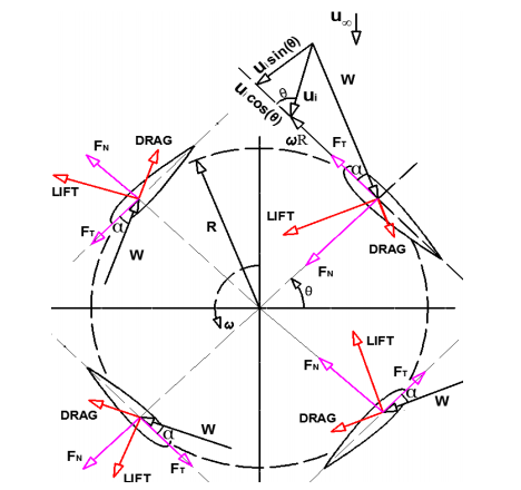
Figure 6. VAWT flow velocities and blades [6]
The rotor of the vehicle will be a sort of VAWT mounted with horizontal axis. The axis of the rotor is perpendicular to the oncoming airflow and blades with an axis, which is parallel to the rotation axis. The aerodynamics is much more complicated than the one of the more conventional propellers such as the ones used for traditional autogyros. According to Bdiago et al. [6], the system can be modelled according to Figure 6.
The normal and tangential force coefficients can be expressed by the following expressions:
${{C}_{n}}={{C}_{L}}\cos \alpha +{{C}_{D}}\sin \alpha $ (11)
${{C}_{t}}={{C}_{L}}\sin \alpha -{{C}_{D}}\cos \alpha $ (12)
where CL is the lift coefficient and CD is the drag coefficient for angle of attack a.
If h is the blade height and c is the blade chord Length, it can be possible to evaluate
$\left\{ \begin{align} {{F}_{N}}=\frac{1}{2}\cdot \rho \cdot {{w}^{2}}\cdot (hc)\cdot {{C}_{n}} \\ {{F}_{T}}=\frac{1}{2}\cdot \rho \cdot {{w}^{2}}\cdot (hc)\cdot {{C}_{t}} \\\end{align} \right.$ (13)
in which the relative velocity w is
$w=\sqrt[{}]{{{\left( {{u}_{i}}\sin \theta \right)}^{2}}+{{\left( {{u}_{i}}\cos \theta +\omega R \right)}^{2}}}$ (14)
Assuming Figure 6 as a reference, thrust on a single blade can be expressed by equation 15.
${{T}_{i}}={{F}_{T}}\cdot \cos \theta -{{F}_{N}} \sin \theta $ (15)
Consequently, the lift force is given by:
${{L}_{i}}={{F}_{T}}\cdot \sin \theta +{{F}_{N}} \cos \theta $ (16)
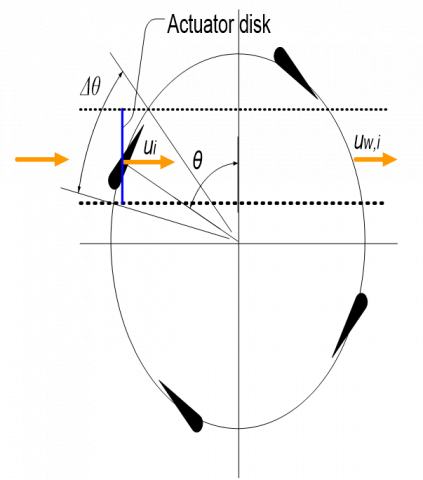
Figure 7. 2D Schema of the stream tube model
Considering a stream tube, it can be possible to determine the average thrust and lift of the system:
${{T}_{avg}}=2\cdot \left( {{n}_{b}}\cdot \frac{\Delta \theta }{\pi }\cdot {{T}_{i}} \right)$ (17)
${{L}_{avg}}=2\cdot \left( {{n}_{b}}\cdot \frac{\Delta \theta }{\pi }\cdot {{L}_{i}} \right)$ (18)
The design of the new passive propeller that can jointly ensure an adequate lift can be produced by making some further considerations.
Considering the rotor of Radius R, it can be possible to determine the external area of the rotor
$A=2\cdot R\cdot L$
and Reynolds number of the rotor.
$\operatorname{Re}=\frac{\rho \cdot {{u}_{o}}\cdot R}{\mu }$
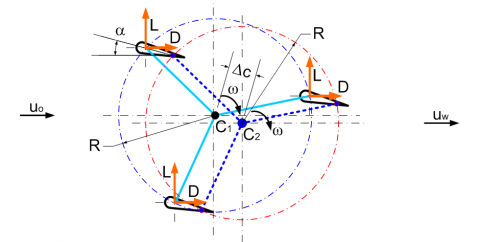
The specific objective of the new rotary wing system is related to the maximization of the aerodynamic lift. This objective requires a redefinition of the geometry of the blades. A definition of a new system that ensures to rotate the blades keeping them parallel during the motion is produced by considering two centres of rotation.
Figure 8. The passive propeller concept
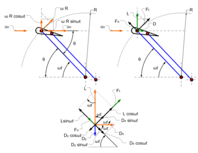
The propeller for the specific aircraft can be assumed to use a new architecture, with two rotation centres. In this case, it can be possible to express the aerodynamic forces. Neglecting the interference between the wings, it the law of motion and the equilibrium of the wing become: The kinetic and dynamic magnitudes of the rotor system are represented in Figure 9.
Figure 9. Kinetic and dynamic magnitudes
Considering a wing that rotates with velocity ω it can be possible to express the two components of velocity of the rotating wing.
$\left\{ \begin{align} {{u}_{wing,x}}=\omega R\cdot \sin \omega t \\ {{u}_{wing,y}}=\omega R\cdot \cos \omega t \\\end{align} \right.$
It can be then possible to determine the two components of the related airspeed:
$\left\{ \begin{align} {{u}_{air,x}}={{u}_{o}}-\omega \cdot R\cdot \sin \omega t \\ {{u}_{air,y}}=-\omega \cdot R\cdot \cos \omega t \\\end{align} \right.$ (19)
From those expressions, it can be possible to express the equations of the aeronautic forces acting on the wing:
$\begin{align} {{D}_{{{u}_{air}},x}}=\frac{1}{2}{{C}_{D,x}}\rho A\cdot u_{x}^{2}=\frac{1}{2}{{C}_{D,x}}\rho A\cdot {{({{u}_{o}}-\omega R\sin \omega t)}^{2}} \\{{L}_{{{u}_{air}},y}}=\frac{1}{2}{{C}_{L,x}}\rho A\cdot u_{x}^{2}=\frac{1}{2}{{C}_{L,x}}\rho A\cdot {{({{u}_{o}}-\omega R\sin \omega t)}^{2}} \\ {{D}_{{{u}_{rot}},y}}=\frac{1}{2}{{C}_{D,y}}\rho A\cdot u_{y}^{2}=\frac{1}{2}{{C}_{D,y}}\rho A\cdot {{(-\omega R\cos \omega t)}^{2}} \\ {{L}_{{{u}_{rot}},x}}=\frac{1}{2}{{C}_{L,y}}\rho A\cdot u_{y}^{2}=\frac{1}{2}{{C}_{L,y}}\rho A\cdot {{(-\omega R\cos \omega t)}^{2}} \\\end{align}$
Figure 10. Graphical analysis of the forces in the different sectors of the wind turbine
According to Figure 10, it can be possible to determine the contribution of the different sectors in order to produce an adequate geometric definition of the pitch of the blades.
Torres and Mueller [7] have directly measured the forces on low aspect ratio (AR) rectangular flat plates for 0.5 ≤ AR ≤ 2 and α ≤ 50°. They have expressed lift coefficient with the expression:
CL =sin α · cos α · (Kp · cos α + ∏ · sin α)
It is possible to write the equations of the forces as a function of the angle of attach by assuming the parabolic model of the relation between CL and CD [8].
${{C}_{D}}={{C}_{D,0}}-{{C}_{Di}}={{C}_{D,0}}+K\cdot {{C}_{L}}^{2}$,
in which CDi is the induced drag and K is given by
$K=\frac{1}{\pi \cdot e\cdot AR}$
where
$AR=\frac{b}{C}=\frac{{{b}^{2}}}{A}$
and e is the Oswald efficiency factor, which is usually between 0.7 and 0.9, and can be determined by the following expression for a straight wing with rectangular area:
$e=1.78\cdot \left( 1-0.045A{{R}^{0.68}} \right)-0.64$
According to [8] and [9], it can be possible to use the following empirical relations for CD and CL at different angles of attach.
${{C}_{L}} = 2\pi \cdot \alpha $
${{C}_{D}}=1.28\cdot \sin \alpha $
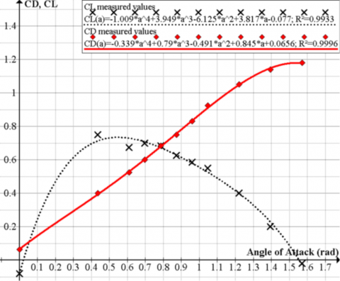
Those simplified expressions allow producing an adequate expression of the forces applied on the plates at low angle of attack. The experimental results by Ortiz [9] allow also considering experimental values that can be easily interpolated.
Figure 11. CL and CD graphs according to Ortiz [9]
$\begin{align} {{F}_{x}}={{D}_{{{u}_{air}},x}}+{{L}_{{{u}_{rot}},x}} =\frac{1}{2}{{C}_{D,x}}\rho A\cdot {{({{u}_{o}}-\omega R\sin \omega t)}^{2}}\pm \frac{1}{2}{{C}_{L,y}}\rho A\cdot {{(-\omega R\cos \omega t)}^{2}} \\ {{F}_{y}}={{L}_{{{u}_{air}},y}}+{{D}_{{{u}_{rot}},y}} =\frac{1}{2}{{C}_{L,x}}\rho A\cdot {{({{u}_{o}}-\omega R\sin \omega t)}^{2}}\pm \frac{1}{2}{{C}_{D,y}}\rho A\cdot {{(-\omega R\cos \omega t)}^{2}} \\\end{align}$
Deriving the above equations, it can be obtained:
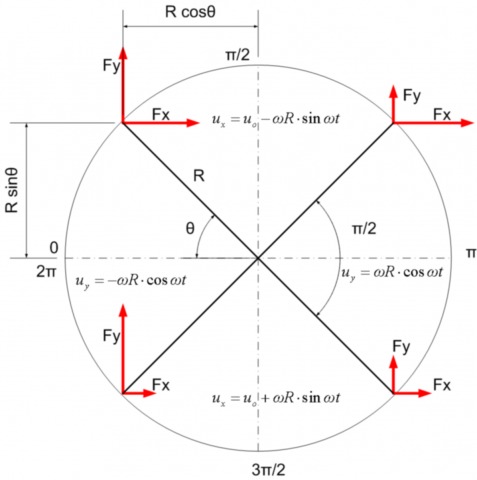
$\begin{align} 0\le \omega t\le \frac{\pi }{2}\to {{M}_{z}}={{F}_{x}}\cdot R\cos \omega t+{{F}_{y}}\cdot R\sin \omega t \\ \frac{\pi }{2}\le \omega t\le \pi \to {{M}_{z}}={{F}_{x}}\cdot R\cos \omega t-{{F}_{y}}\cdot R\sin \omega t \\ \pi \le \omega t\le \frac{3\pi }{2}\to {{M}_{z}}=-{{F}_{x}}\cdot R\cos \omega t-{{F}_{y}}\cdot R\sin \omega t \\ \frac{3\pi }{2}\le \omega t\le 2\pi \to {{M}_{z}}=-{{F}_{x}}\cdot R\cos \omega t+{{F}_{y}}\cdot R\sin \omega t \\\end{align}$
From the above equations, it is immediate to determine the conditions for the optimal configuration of a variable pitch system. The second condition that must be satisfied is the condition of a positive contribution to lift that means Ry>0, that ensures a positive lift.
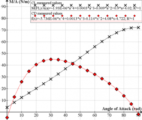
Figure 12. Evaluation of the absolute value of the torque by Fx and Fy on 90° rotation for different angle of attack at 10m/s, R=1 m
It can be possible to determine the optimal average angle of the wings into different sectors. In particular, it has been assumed a max rotation speed about 100 rpm and a radius of the cylinder of the blades of 1m.
Figure 13. Average angles of attack in the different sections of the rotating wing. Results are obtained assuming the condition of maximum lift and avoiding the stall condition
By the above evaluation at different velocities, it is possible to evaluate the condition that allows both the production of energy by rotation and an adequate lift. A possible solution is presented in Figure 13, which is intended to maximize the lift during the rotation. The forces, which are produced by each blade in a complete rotation at a reference cruise speed of 10 m/s, are then equal to the values reported into table 1.
Table 1. Preliminary evaluation for the specific considered configuration of the system at different speeds
|
Lift |
78.26 |
N/(blade m2) |
|
Drag |
66.54 |
N/(blade m2) |
|
Torque |
31.78 |
N/(blade m) |
|
Max Power to generator |
1271.22 |
W/(blade m2) |
|
Power for advancement |
1330.86 |
N/(blade m2) |
Those results even if not completely optimized allow assessing a preliminary feasibility of the system. Considering the results in Figure 12, it is then possible to determine the optimal trajectory of the blades and can be possible to design the piloting cam or mechanism. Further configurations can be experimented.
It can be assumed an ultralight configuration that can be considered competitive with actual autogyros, such as MTO-Free No Limits [10], two-seater autogyro. It is then possible to determine the main characteristics of the necessary rotors.
Table 2. MTO-free no limits data [10]
|
L x W x H: |
5,1 m x 1,9 m x 2,7 m |
|
Empty weight: |
240 kg |
|
MTOW: |
450-500 kg |
|
Engine: |
Rotax 912 ULS | 914 UL |
|
Takeoff distance*1: |
60 m | 50 m | tbd |
|
Max endurance*2: |
4,6 h | 4,1 h | tbd |
|
Max range*2: |
510 km | 450 km | tbd |
|
Cruise speed: |
120 km/h |
|
Max speed: |
150 km/h |
|
Fuel capacity: |
65 ltr |
|
Compliant with: |
BUT, ASRA |
|
*1: typical aircraft configuration, 1 pilot (80kg), 40 ltr fuel, 2000 ft MSL *2: typical aircraft configuration, 1 pilot (80kg), max fuel, 2000 ft MSL |
|
Assuming a diameter of the rotor of 1m it is possible to determine the dimensions of the blades by considering the unitary values, which have been determined before.
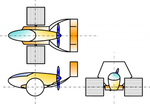
Figure 14. General architecture of the aircraft
Table 3. Calculation of the energetic and geometric properties of the blades.
|
Speed |
36.00 |
54.00 |
72.00 |
90.00 |
108.00 |
126.00 |
144.00 |
km/h |
|
Speed |
10.00 |
15.00 |
20.00 |
25.00 |
30.00 |
35.00 |
40.00 |
m/s00 |
|
Avg. Lift of a blade |
78.26 |
176.09 |
313.04 |
489.13 |
704.34 |
958.69 |
1252.16 |
N/(blade m2) |
|
Avg. Drag of a blade |
66.54 |
149.72 |
266.16 |
415.88 |
598.86 |
815.12 |
1064.64 |
N/(blade m2) |
|
Torque |
31.78 |
71.51 |
127.12 |
198.63 |
286.02 |
389.31 |
508.48 |
N/(blade m) |
|
Power to generator |
1144.10 |
3861.33 |
9152.78 |
17876.53 |
30890.65 |
49053.20 |
73222.27 |
W/(blade m2) |
|
Power for advancement |
1330.86 |
4491.65 |
10646.88 |
20794.69 |
35933.22 |
57060.62 |
85175.04 |
W/(blade m2) |
|
Required area of wings |
62.68 |
27.86 |
15.67 |
10.03 |
6.96 |
5.12 |
3.92 |
m2 |
|
Area of one blade |
7.83 |
3.48 |
1.96 |
1.25 |
0.87 |
0.64 |
0.49 |
m2 |
|
Chord of the blades |
2.61 |
1.16 |
0.65 |
0.42 |
0.29 |
0.21 |
0.16 |
m |
By considering the aircraft architecture in Figure 14, it can be possible to determine the main characteristics of the rotors.
Assuming a cruise speed of (25 m /s and 90 km/h), it is necessary to determine the minimum chord of the blades that results 0.42 m.
This blades dimension allow an optimal lift at the defined cruise speed and by correcting the geometry of the rotary wing will require a power of around 23 kW for flight. This configuration will also ensure an electric cogeneration of 80% of the energy needs for advancing.
By considering equation (1), it can be possible to determine the equation of motion. In particular, the energy equation of the vehicle will allow determining the flight mechanics of the system.
Comparing the results against Betz model, the total incident power on the disk can be expressed. The area of the disk is equal to radius multiplied by span of the disk. The max power generated by the wind at the considered speed is 31,250 W. Considering the maximum cogeneration efficiency that is expected by the ideal turbine it can be possible to compare the efficiency against Betz efficiency. In particular the proposed system has a generation capability of about 57.6% that is effectively lower than Betz limit (59%), demonstrating that the results are in line with theory.
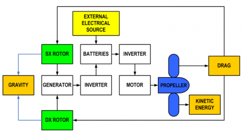
Further analysis will relate to the energy analysis of the system. The power equation found in traditional bibliography, which have been cited in the preceding paragraph, can be improved by a more accurate analysis according to EMIPS (Exergetic Material Input per Unit of Service) [11] as corrected by Trancossi [12, 13].
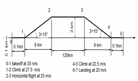
A schema of the powertrain indicating the different losses is provided in Figure 15. Losses depend on the flight condition in which the vehicle operates. Energy balance against helicopters has been evaluated on a reference mission profile (Figure 16).
Figure 15. Energy balance schema
Figure 16. Reference mission profile
According to the mission profile, which has been indicated, it can be possible to identify the energy consumption (Table 3). Take off space is limited to 90 m and the same for landing space.
Energy analysis has been performed according to the general flight mechanics equations of an aircraft by Hull [12] as corrected by Trancossi [13].
Table 4. Energy consumption and cogeneration potential
|
|
L |
v |
T |
Energy |
Cogen |
Energy used (kJ) |
|
0-1 |
0.1 |
30.0 |
6.7 |
1600.0 |
1120.0 |
480.0 |
|
1-2 |
9.5 |
27.5 |
345.0 |
10349.3 |
7244.5 |
3104.8 |
|
2-3 |
120.0 |
25.0 |
4800.0 |
100800.0 |
75600.0 |
25200.0 |
|
3-4 |
9.5 |
22.5 |
421.6 |
6324.6 |
5059.6 |
1264.9 |
|
4-5 |
0.1 |
20.0 |
10.0 |
110.0 |
93.5 |
16.5 |
The paper clearly demonstrates a preliminary feasibility of a new autogyro concept that uses two passive cyclorotors on the side of the vehicle. This new architecture does not require any other aerodynamic control except a braking system that can reduce the speed of the rotors allowing steering the system.
The actual vehicle has the potential of producing a very high cogeneration capability with respect to any other presents a very high efficiency. The actual results demonstrate that the architecture of the system allows producing a vehicle concept that can be energy efficient and functional in particular at low speed. The results demonstrates that the proposed system respect the Betz limit. The preliminary definition of the wings and of the rotors has been produced and a preliminary energy assessment that clearly demonstrates that the presented innovative aircraft architecture could present major energy advantages. In particular, the proposed configuration reduces also well-known problems that affect the traditional autogyros such as the eccentricities in the generation of aerodynamic forces such as the one generated by the vertical turbine.
|
CD |
drag coefficient (-) |
|
CL |
lift coefficient (-) |
|
Ɵ |
angle (rad) |
|
Ω |
angular velocity (rad/s), (1/s) |
|
a |
angle of attack (º). |
|
r |
density (kg/m3) |
|
ω |
angular velocity, (rad/s) |
|
A |
area (m2) |
|
D |
drag (N) |
|
E |
energy (J) |
|
L |
lift (N) |
|
R |
radius (m) |
|
g |
gravitational acceleration (m.s-2) |
|
h |
altitude (m) |
|
m |
mass (kg) |
|
p |
pressure (Pa) |
|
t |
time (s) |
|
u |
air speed (m/s) |
|
N |
normal (forces) |
|
T |
tangential (forces) |
|
avg |
average |
|
b |
body of the aircraft |
|
n |
normal |
|
o |
far field velocity |
|
r |
rotor |
|
t |
tangential |
|
w |
downwash speed |
|
x |
x axis |
|
y |
y axis |
[1] Leishman J.G. (2004). Development of the autogiro: A technical perspective, Journal of Aircraft, Vol. 41, No. 4, pp. 765-781. DOI: 10.2514/1.1205
[2] De La Cierva J. (1930). The autogiro, The Journal of the Royal Aeronautical Society, Vol. 34, No. 239, pp. 902-21. DOI: 10.1017/S0368393100115093
[3] Glauert H. (1927). The theory of the autogyro, Journal of the Royal Aeronautical Society, Vol. 31, No. 198, pp. 483-508. DOI: 10.1017/S0368393100133206
[4] Zhuang N., Xiang J., et al. (2014). Calculation of helicopter maneuverability in forward flight based on energy method, Computer Modelling & New Technologies, Vol. 18, No. 5, pp.50-54.
[5] Okulov V.L., Sørensen J.N. (2010). Maximum efficiency of wind turbine rotors using Joukowsky and Betz approaches, Journal of Fluid Mechanics, Vol. 649, pp. 497-508. DOI: 10.1017/S0022112010000509
[6] Biadgo M.A., et al. (2013). Numerical and analytical investigation of vertical axis wind turbine, FME Transactions, Vol. 41, No. 1, pp. 49-58.
[7] Torres G.E., Mueller T.J. (2004). Low aspect ratio aerodynamics at low Reynolds numbers, AIAA Journal, Vol. 42, pp. 865-873.
[8] McCormick B.W. (1995). Aerodynamics; Aeronautics; and Flight Dynamics, John Wiley.
[9] Ortiz X., Hemmatti A., Rival D., Wood D. (2012). Instantaneous forces and moments on inclined flat plates, 7th International Colloquium on Bluff Body Aerodynamics and Applications (BBAA7), pp. 2-6.
[10] MTO Free Technical data, from https://www.auto-gyro.com/en/Gyroplane/AutoGyro-Models/MTOfree/
[11] Dewulf J., Van Langenhove H. (2003). Exergetic material input per unit of service (EMIPS) for the assessment of resource productivity of transport commodities, Resources Conservation and Recycling, Vol. 38, No. 2, pp. 161-174.
[12] Trancossi M. (2016). What price of speed? A critical revision through constructal optimization of transport modes, International Journal of Energy and Environmental Engineering, Vol. 7, No. 4, pp. 425-448.
[13] Hull D.G. (2007). Fundamentals of airplane flight mechanics, ISBN: 978-3-540-46571-3.
[14] Trancossi M., Stewart J., Pascoa J.C. (2016). A New propelled wing aircraft configuration, ASME 2016 International Mechanical Engineering Congress and Exposition, American Society of Mechanical Engineers, pp. V001T03A048-V001T03A048. DOI: 10.1115/IMECE2016-65373