OPEN ACCESS
The area of domestic heating and cooling is nowadays a key sector in the energy policies pursued by the European Union, since about 30% of energy consumption in the EU countries is due to thermal comfort in buildings. To achieve the reduction of fossil fuels consumption one solution is to optimize the use of the energy having an efficient management of the heating plants. A dynamic approach is therefore needed, since energy saving actions are possible only with the knowledge of the behavior in time of the different elements of the plant. In this paper, the development of a dynamic model for buildings heating plants is described. The model, validated by means of a comparison with measured data, allows to simulate the variation in time of some key parameters and to describe the behavior of the whole system for varying boundary conditions. Some parametric studies are presented in order to better describe the capabilities of the model.
heating plants, buildings, numerical models, dynamic models, MATLAB/simulink
In the current technique is more and more important to forecast the behavior of heating plants as a function of external conditions and heat load, both for operational planning and for operational optimization [1, 2]. Expectation of reliable and cost-effective performance improvements can be met only through the development of new simulation methods, able to predict the evolution over time of the different key variables of the heating system [3, 4, 5, 6]. The present challenge is to switch from well-established stationary design approach, to dynamic modelling, in order to analyze for each system component the behavior over time.
This increasing forecast capacity need follows heating plants evolution. Reduction of pollutant emissions, indoor comfort conditions, operating reliability and reduced fuel consumption are all important goals that require accurate and effective forecasting models. For this reason, a lot of effort has been put to overcome criticalities in heating plants dynamic modeling caused by systems complexity, uncertainties in operating conditions, and lack of data for model validation [7, 8]. In spite of these difficulties, several outcomes attest the effectiveness of heating plants dynamic simulation and the possibilities that this technique offers of a new, more operative, heating systems control.
Some Authors followed the path of self-produced software applications, ranging from lumped parameters models [9], to dynamic models mostly focused on building physical parameters [10], until an enhanced capacity of simulating the integration between plant and building [11].
Besides, data flow graphical programming language tools, such as the MATLAB/Simulink environment, are largely used to dynamically simulate heating plants and analyze their characteristics in terms of temperature control and efficiency. Exhaustive reviews are given in ref. [12] with specific reference on MATLAB/Simulink and in ref. [13] for different kinds of programming environment. Tools like IDA and SPARK allow to create general models in which a certain particular condition is developed and analyzed only weather a specific set of input parameters occur. Moreover, the simulation of the behavior of each single component is possible through an “input/output” approach [14].
Recent developments see an improved integration of building and plant dynamic simulation, aiming to a better comprehension of the effect of all external conditions on energy consumption and environmental impact. Cockoft et al. [15] developed the modelling of a heating plant with a detail including components such as flow control and energy conversion devices and controllers. The study demonstrates the ability of detailed building and plant modelling to reveal unexpected insights into how real control systems perform in combination with other plant items and in different building types, including estimation of their influence on annual energy consumption. The whole-building simulation program TRNSYS was used by Dorer and Weber [16] in order to conduct a performance assessment study for a number of micro-CHP systems and residential buildings. Through the dynamic modelling of heating plants integrated in single and multi-family houses of different energy standard levels a thorough consumption assessment was performed, so fully exploiting the simulation potential. Integration between plant and building modelling is also the focus of Testi et al. [17], who applied dynamic simulation to radiant systems coupled with a modulating heat pump. The outcome shows how different control strategies can be compared, so that optimal design of new systems and energy audit of existing buildings can be implemented.
The present paper describes the development of a numerical model, implemented in MATLAB/Simulink environment, aiming to dynamically simulate the behavior of single building heating systems, and address its validation through the comparison with experimental data logged for a real building heating plant. Finally, the application of the model to test cases is reported for the purpose to testify its capabilities. These results show how dynamic modelling permits to analyze the behavior of building-heating systems and to evaluate their performance. In comparison with stationary models, the dynamic ones give the important possibility to study the evolution over time of the plant and to pursue, in a more effective way, its optimization.
In this paper, a central heating system of a building is simulated by means of a dynamic numerical model.
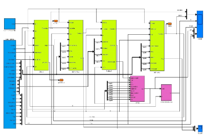
The model is developed in MATLAB/Simulink and is represented in Fig. 1. Here the green blocks represent the regulation of the plant (i.e. boiler, heaters, supply and return pipelines) while pink blocks represent the building and the thermostatic valves and the blue blocks are the inputs and the outputs of the model [18].
Figure 1. Sketch of the model
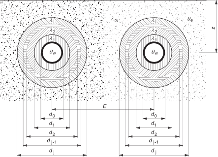
Figure 2. Two pipes installed in the masonry [20]
The operating parameters of the different components of the plant are given as inputs to the model in the form of time dependent curves. This allows to have a fully dynamic simulation, in which the user can also take advantage from a number of configurable settings and controls that allow to analyze different plant configurations in a quick and easy way.
The various components of the model are briefly described hereafter.
2.1 Pipes
In order to be simulated, the inputs needed for the pipes are internal and external diameters, density and specific heat of the material the pipe is made of, thickness of the material wrapping around the pipes and separating them from the external environment (soil and/or masonry), thermal conductivities of the materials and the external heat transfer coefficient, the overall heat exchange coefficient, the mass of water in the pipes, the thermal inertia of the system made by pipe/masonry and the internal heat exchange surface.
According to UNI/TS 11300-2:2014 Standard [19], the transmittance is calculated by means of the following Eq (1):
${{U}_{i}}=\frac{\pi }{\sum\limits_{j=1}^{n}{\frac{1}{2\cdot {{k}_{j}}}\cdot \ln \frac{{{d}_{j}}}{{{d}_{j}}-1}+\frac{1}{2\cdot {{k}_{G}}}\cdot \ln \frac{4\cdot z}{{{d}_{n}}}+\frac{1}{2\cdot {{k}_{G}}}\cdot \ln \sqrt{1+\frac{4\cdot {{z}^{2}}}{{{E}^{2}}}}}}$ (1)
where n is the number of insulation layers, dj the external diameter of insulation layer j starting from the inner one [m], d0 the external diameter of the pipe, dn the whole external diameter of the insulated pipe, kj the conductivity of the insulation layer j, kG the conductivity of the masonry (assumed equal to 0.7 if there is not any available information), z is the installation depth (assumed equal to 0.1 if no information is available) and E is the center distance of the pipes as reported in Fig. 2.
The LMTD cannot be calculated as the temperature of the surrounding environment is not known: for this reason the pipe is split into linear sections, applying for each one Eq(2):
$\overline{T}=\frac{{{T}_{in}}+{{T}_{out}}}{2}$ (2)
From the balance equation between the fluid and the pipes, it is possible to obtain
${{\left( M\cdot c \right)}_{w}}\cdot \frac{d\bar{T}}{dt}=\dot{m}\cdot {{c}_{W}}\cdot \left( {{T}_{in}}-{{T}_{out}} \right)-{{h}_{i}}\cdot {{A}_{i}}\cdot \left( \bar{T}-{{T}_{P}} \right)$ (3)
where (M∙c)w is the thermal capacity of the water, ṁ is the mass flow rate of fluid flowing in the system and regulated by thermostatic valves, hi the heat transfer coefficient between the fluid and the inner surface of the tubes, Ai the inner surface of the tubes.
Finally, from the general equation of balance between pipes and external environment, we obtain Eq. (4):
${{\left( M\cdot c \right)}_{P}}\cdot \frac{d{{T}_{P}}}{dt}={{h}_{i}}\cdot {{A}_{i}}\cdot \left( \bar{T}-{{T}_{P}} \right)-{{\left( U\cdot A \right)}_{ext}}\cdot \left( {{T}_{P}}-{{T}_{ext}} \right)$ (4)
where (M∙c)p is the thermal capacity of the pipe and Text is the outdoor temperature.
2.2 Boiler
The boiler block is power controlled by means of the climatic curve obtained taking into account the lowest design temperature and the return temperature of the plant. If the water circulation is active we have
${{\left( M\cdot {{c}_{{}}} \right)}_{b}}\cdot \frac{dT}{dt}={{\dot{m}}_{gas}}\cdot {{H}_{i}}-{{\dot{m}}_{w}}\cdot \left( {{T}_{supp}}-{{T}_{ret}} \right)$ (5)
where (M∙c)b is the thermal capacity of the boiler and Hi is the lower heating values of the fuel (natural gas).
2.3 Radiators
The model of the radiators is based once again on the conservation of energy, by means of Eq(6):
${{(M\cdot c)}_{R}}\cdot \frac{d{{T}_{R}}}{dt}=\dot{m}\cdot {{c}_{{{W}_{{}}}}}\cdot ({{T}_{in}}-{{T}_{out}})-{{h}_{e}}\cdot {{A}_{e}}\cdot ({{T}_{R}}-{{T}_{env}})$ (6)
where (M∙c)R represents the thermal capacity of the heating elements, Tr is the arithmetic mean between Tin and Tout, ṁ is the mass flow rate, he the heat transfer coefficient between fluid and external environment, Ae the heat exchange surface of the external radiators and Tenv the ambient temperature in the building, depending on the power delivered from the radiators and the characteristics of the building itself.
Every radiator is equipped with a thermostatic valve simulator which avoids unnecessary overheating switching off the water flow rate, thus decreasing the power of the boiler and obtaining a noticeable energy saving.
2.4 Building
The building is simulated by means of physical and geometrical characteristics, taking into account its exposure and a term for accumulation represented by the thermal inertia of the system.
The analysis takes into account the incoming and outgoing heat fluxes [19]:
${{\left( M\cdot c \right)}_{B}}\cdot \frac{d{{T}_{env}}}{dt}=\sum{q}$ (7)
The term Σq is given by the sum of the following contributions:
${{q}_{t}}=K\cdot S\cdot \left( {{T}_{env}}-{{T}_{ext}} \right)$ (8)
${{q}_{v}}={{C}_{v}}\cdot ({{T}_{env}}-{{T}_{ext}})$ (9)
${{q}_{sol}}=K\cdot {{R}_{ext}}\cdot S\cdot \varepsilon \cdot I\cdot b$ (10)
Here, qt represents heat flux leaving the building, qv the heat flux for ventilation and qsol the incoming heat flux due to solar gains. In Eq(8, 9, 10) K is the thermal transmittance of the walls, S the heat exchange surface of the building, Cv is the heat capacity due to ventilation, ε the emissivity of the outer surface of the building, I the solar irradiance and b is a correction factor that takes into account exposure and shading. Internal gains are applied according to UNI/TS 11300 Standard.
The validation of the model was carried out comparing the results obtained by the simulations with quantities measured in an existing 5 storey Italian condominium located in Asti, Italy. The delivery system uses aluminum radiators with a low thermal inertia equipped with on/off thermostatic valves. Several simplifications were made in order to implement the 20 different apartments of the building: one example is that the model simulates a single apartment with 6 radiators, thus obtaining the 5% of the total flow rate circulating in the plant. This leads to the hypothesis of considering each apartment with the same structural characteristics and physical properties: even if this is of course a simplification, as apartments on the first and top floor have completely different behaviours if compared to the ones located in the mid floors, the results are quite satisfactory.
Simulations regarding supply temperature, return temperature and mass flow rate were compared with the measured values for two days. The results obtained have been analyzed in terms of the fraction of data predicted to within ±20%, called λ, and the mean absolute percent error, MAPE, evaluated trough Eq(11):
$MAPE=\frac{1}{N}\sum\limits_{i=1}^{N}{\left| \frac{predict.value-exp.value}{exp.value} \right|}%$ (11)
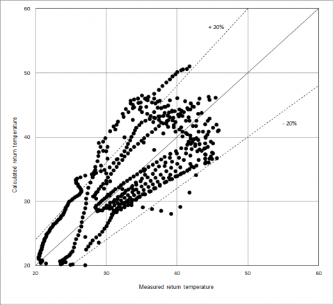
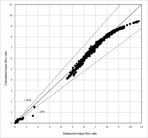
Figures 3-5 show the comparison between measured and predicted temperature values for supply temperature, return temperature and mass flow rate; the dotted lines indicate a difference between predicted and experimental values of ±20%. The absolute mean error resulted equal to 4.8°C for supply temperature and 4.6°C for return temperature.
The values of MAPE and λ in reference to the whole data set of the supply temperature are respectively equal to 12.9% and 84.3%; for return temperature, these values are respectively 14.1% and 80.0%. Considering the mass flow rate, the values of MAPE and λ temperature are respectively equal to 8.7% and 87.4%.
Figure 3. Comparison between measured and predicted supply temperature
Figure 4. Comparison between measured and predicted return temperature
Figure 5. Comparison between measured and predicted mass flow rate
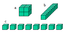
The model was applied to several different configurations in order to test its capability in describing new scenarios in terms of plant management, building envelope and geometry. An ideal building was considered, located in Genoa, with a volume of 512 m3. It is assumed that the building has three floors with four radiators per floor. A typical January day was simulated, using as input values of temperature and irradiance real data obtained from the meteorological station of the Department of civil, chemical and environmental engineering of the University of Genoa. Several hypotheses have been made: pipes are made of uninsulated copper and are inserted in masonry walls; radiators are made of cast iron; thermostatic valves are of the on/off kind; the boiler is activated when the flow temperature is equal to 40°C. The aspect ratio of the ideal building considered varies according to the following figure 6 and table 1.
Figure 6. Different configurations tested
Table 1. Aspect ratios
|
Case |
A |
A/V |
|
a |
387 |
0.75 |
|
b |
544 |
1.0625 |
|
c |
768 |
1.5 |
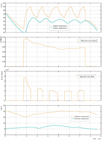
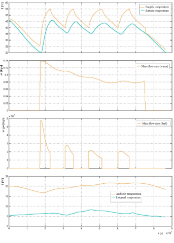
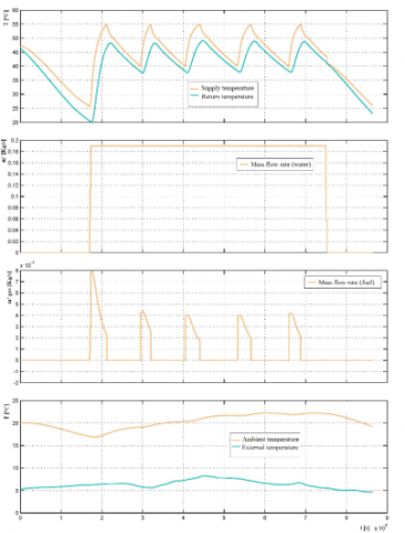
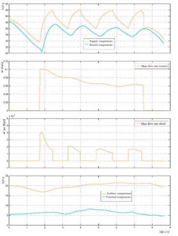
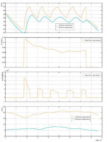
The obtained results (Fig. 7-14) show the time history of supply and return temperature, water (regulated by thermostatic valves) and fuel mass flow rates, ambient internal temperature of the building and external temperature. When the supply temperature reaches 55 °C a “relay” command disables the boiler until the temperature drops below 40 °C, moment in which the boiler is reactivated. The fluid flow is regulated by thermostatic valves on each radiator allowing the passage of a predefined amount of fluid in function of the temperature that is established within the building. This allows to avoid the overheating of the building and the consequent unnecessary energy waste. In the end, boiler and pump are switched off and all the temperature curves show a decreasing trend.
Since energy efficiency depends also on the geometrical shape of the building, as expected (see Figures 8-10) the smaller is the surface of the building, the less energy will be lost. Corners, projections and recesses considerably increase the size of the surface.
As it can be seen from figures 9 and 10, in some configurations the trend of the temperature inside the building is considerably lowered, until it cannot even reach the desired 20 °C because the dispersions are too high. This is due to a different slope of the cooling curve, mainly due to the heat exchange between the heating elements and the building and by the increase in the flow regulated by the thermostatic valves, resulting in an increase of the power needed to heat up a larger amount of water.
Figures 10 and 11 show that the model correctly represents the behavior of the various plant components in the case of a variation of the mass flow rate of fluid circulating in the plant, being kept constant the control curve of the thermostatic valves. This corresponds to a variation in the activity of the boiler and of the room temperature despite the presence of the thermostatic valves. A greater activity of the boiler and an increase in temperature inside the rooms result in a higher flow rate, while the opposite happens in case of a reduction of the flow rate.
As a further example, figure 12 shows the behavior of the various main parameters considered in the case the plant is powered by a constant flow rate, which corresponds to the maximum in the presence of valves. As it can be noted, the boiler activity of course increases, but more importantly, with all other parameters kept constant, the ambient temperature inside the building excessively increases.
Figure 7. Simulation results for A/V=0.75
Figure 8. Simulation results for A/V=1.0625
Figure 9. Simulation results for A/V=1.5
Figure 10. Simulation results for an increased water mass flow rate
Figure 11. Simulation results for a decreased water mass flow rate
Figure 12. Simulation results for constant water mass flow rate
Figure 13. Simulation results for an increased thermal inertia of the pipes
Figure 14. Simulation results for a low thermal inertia emission system
In order to underline how the model is particularly oriented to the simulation of plant components, two more analyses were carried out.
The first one is aimed to reduce heat loss along pipes (at first considered uninsulated as previously described). This is possible simulating the addition of insulating material and thus increasing the thermal resistance of the whole system represented by pipes and the surrounding insulating material. This leads to a reduction of the slope of the supply and return temperature curves when the boiler is not active (see Fig. 13), and this behavior is also reflected on the internal temperature of the rooms. As a consequence, a reduction of fuel flow (and therefore of the power delivered by the boiler) can be noticed.
The last analysis described here is about the possibility of changing the thermal inertia of the emission system. Cast iron radiators are substituted with aluminium ones with a faster response to temperature changes. A climate such as the Italian one, characterized by strong thermal excursions throughout the day and a moderate sun irradiation, makes a system able to intervene as quickly as possible by partially subtracting the heat input to the emission system extremly desirable. In this way, a home equipped with low thermal inertia emission systems can optimize the free heat inputs (also due to household appliances, people, etc.) and contribute to energy savings.
As it can be seen by figure 14, the system responds more quickly to ambient temperature changes inside the building. On one hand, it can be seen a lower ambient temperature value when the boiler is not active, due to a more abrupt cooling of the system. On the other hand, less time is needed to achieve the desired ambient temperature, which translates in a greater comfort. The boiler intervenes more frequently switching on and off due to the more rapid variations of the whole system.
A dynamic numerical model to simulate the heating plant of a building was developed and validated. The validation showed a good agreement between simulated and measured values of supply and return temperatures and water mass flow rate, confirming the validity of the software and the importance of a correct formulation of the study, from the collection of climate data to the precise definition of the geometry and thermo-physical properties of studied building.
Subsequently, the model was applied to different building configurations, allowing the simulation of the thermal behavior of the whole plant-building system at the varation of some main parameters.
The parametric study of the building system allowed to reach the following conclusions. The model:
- is a good tool for the comparable evaluation of different energy retrofitting interventions;
- is easily adaptable to other plant solutions;
- allows to analyze the heating requirements of the building, dynamically, taking into account all the variables involved.
Stationary tools, in fact, are most commonly used in the design phase, have the advantage of simplicity but do not assess the differences that exist, for example, between a building that is simply compliant with the regulatory limits and one designed to appropriately respond to the natural and climatic environmental stresses.
|
A |
surface |
|
b |
correction factor for exposure and shading |
|
c |
specific heat |
|
C |
heat capacity |
|
d |
diameter |
|
E |
center distance of the pipes |
|
h |
heat transfer coefficient |
|
Hi |
lower heating value |
|
I |
solar irradiance |
|
k |
thermal conductivity |
|
K |
thermal transmittance |
|
ṁ |
mass flow rate |
|
M |
mass |
|
MAPE |
mean absolute percent error |
|
n |
number of insulation layers |
|
q |
heat flux |
|
S |
heat exchange surface of the building |
|
T |
temperature |
|
U |
transmittance of two insulated pipes in a wall |
|
V |
volume |
|
z |
installation depth |
|
Greek symbols |
|
|
ε |
emissivity of the outer surface of the building |
|
λ |
fraction of data predicted to within ±20% |
|
Subscripts |
|
|
b |
boiler |
|
B |
building |
|
e |
external |
|
G |
masonry |
|
gas |
gas |
|
i |
ith element |
|
in |
inlet |
|
j |
jth element |
|
out |
outlet |
|
p |
pipe |
|
r |
radiator |
|
Sol |
solar |
|
T |
temperature |
|
v |
ventilation |
|
w |
water |
[1] Benonysson A., Bøhm B., Ravn H.F. (1995). Operational optimization in a district heating system, Energy Conversion and Management, Vol. 36, pp. 297–314. DOI: 10.1016/0196-8904(95)98895-T
[2] Zhu S., Guo S., (2011). A study of predictive control of energy-saving of heating process, Advanced Materials Research, Vol. 328-330, pp. 1810-1813. DOI: 10.4028/www.scientific.net/AMR.328-330.1810
[3] Lo Cascio E., Borelli D., Devia F., Schenone C. (2017). Future distributed generation: An operational multi-objective optimization model for integrated small scale urban electrical, thermal and gas grids, Ener Convers Manage, Vol. 143, pp. 348 359. DOI: j.enconman.2017.04.006
[4] Lo Cascio E., Borelli D., Devia F., Schenone C. (2017). Residential Building Retrofit through Numerical Simulation: A Case Study, Ener Proc, Vol. 111, pp. 91-100. DOI: 10.1016/j.egypro.2017.03.011
[5] Di Bella A., Granzotto N., Elarga H., Semprini G., Barbaresi L., Marinosci C. (2015). Balancing of thermal and acoustic insulation performances in building envelope design, Proceedings of INTER-NOISE 2015, pp. 1209-1219. DOI: 10.13140/RG.2.1.1435.9122
[6] Tagliafico L.A., Cavalletti P., Fabbri C., Scarpa F. (2016). Dynamic behaviour and control strategy optimization for conventional heating plants in buildings, Int J Heat Tech, Vol. 34, pp. S505-S511. DOI: 10.18280/ijht.34Sp0244
[7] Ben-Nakhi A., Aasem E.O. (2003). Development and integration of a user friendly validation module within whole building dynamic simulation, Ener Convers Manage, Vol. 44, pp. 53-64. DOI: 10.1016/S0196-8904(02)00039-0
[8] D’alessandro F., Bianchi F., Baldinelli G., Rotili A., Schiavoni S. (2017). Straw bale constructions: Laboratory, in field and numerical assessment of energy and environmental performance, J Build Engr, DOI: 10.1016/j.jobe.2017.03.012
[9] Hudson G., Underwood C.P. (1999). A Simple building modelling procedure for MATLAB/SIMULINK, 6th International IBPSA Conference, Kyoto, Japan, pp. 777-783.
[10] Nannei E., Schenone C. (1999). Thermal transients in buildings: Development and validation of a numerical model, Energy and Buildings, Vol. 29, No. 3, pp. 209-215. DOI: 10.1016/S0378-7788(98)00060-7
[11] Mendes N., Oliveira G.H.C., Araújo H.X. (2001). Building thermal performance analysis by using Matlab/Simulink, 7th International IBPSA Conference, Rio de Janeiro, Brazil, pp. 473-480.
[12] Riederer P. (2012). Matlab/Simulink for building and HVAC Simulation - State of the art, 9th International IBPSA Conference, Montréal, Canada, pp. 1019-1026.
[13] Kramer R., Schijndeln J., Schellen H. (2012). Simplified thermal and hygric building models: A literature review, Frontiers of Architectural Research, Vol. 1, No. 4, pp. 318-325. DOI: 10.1016/j.foar.2012.09.001
[14] Sowell E.F., Haves V. (2001). Efficient solution strategies for building energy system simulation, Energy and Buildings, Vol. 33, No. 4, pp. 309-317. DOI: 10.1016/S0378-7788(00)00113-4
[15] Cockroft J., Kennedy D., O'Hara M., Samuel A., Strachan P., Tuohy P. (2009). Development and validation of detailed building, plant and controller modelling to demonstrate interactive behaviour of system components, IBPSA 2009 - International Building Performance Simulation Association, pp. 96-103.
[16] Dorer V., Weber A. (2009). Energy and CO2 emissions performance assessment of residential micro-cogeneration systems with dynamic whole-building simulation programs, Ener Conv Manage, Vol. 50, pp. 648-657. DOI: 10.1016/j.enconman.2008.10.012
[17] Testi D., Schito E., Tiberi E., Conti P., Grassi W. (2015). Building energy simulation by an in-house full transient model for radiant systems coupled to a modulating heat pump, Energy Procedia, Vol. 78, pp. 1135-1140, 6th International Building Physics Conference, IBPC 2015.
[18] Borelli D., Repetto S., Schenone C. (2014). A dynamic model for building heating plants, in Latest trends in applied and theoretical mechanics, Proceedings of the 10th International Conference on Applied and Theoretical Mechanics (MECHANICS '14), pp. 84-92.
[19] Energy performance of buildings - Part 2: Evaluation of primary energy need and of system efficiencies for space heating, domestic hot water production, ventilation and lighting for non-residential buildings, UNI/TS Standard 11300-2, 2014.