OPEN ACCESS
The optimization of the performance of air conditioning systems is mandatory in order to minimize costs by ensuring the attainment of specific thermo-hygrometric conditions of controlled environments at the same time. The aim of the present work is the analysis of the process parameters that play a fundamental role in the conditioning process of controlled microclimates. Starting from a predictive mathematical model that was developed to study the performance of air-conditioned environments, two upgrades are presented by implementing two separate control systems. The first one is based on an adjustable airflow rate and the other on an adjustable inlet temperature of the controlled environment. The first model estimates the energy consumption in terms of heating/cooling and humidification/dehumidification energy and reheat (when such process occurs) with an adjustable airflow rate computed by performing a heat transfer balance of the microclimate environment for a given inlet temperature. In the second model, the energy consumption is evaluated by keeping the airflow rate quasi-constant and adjusting the inlet temperature based on a thermal energy balance of the controlled environment. The results obtained with the two models have been compared under several climatic and set-point (comfort) conditions, thus assessing the advantages and disadvantages of both models.
dynamic simulation, air conditioning, control systems, microclimate, energy efficiency
The air conditioning systems of indoor environments require high performance in terms of energy consumptions in order to minimize costs by ensuring the attainment of specific thermo-hygrometric conditions. The improvement of the energy performance of conditioning plants requires a careful analysis of the energy system and of the different process parameters that affect the performance of such a system. The system components should be properly designed and optimized in order to reduce the energy consumption and pollutant emissions.
A predictive mathematical model has been already developed in Ref. [1] in order to study the performance of the air conditioning systems for controlled microclimates. The authors provided an estimate of the energy consumptions in terms of heating/cooling and humidification/dehumidification energy and reheat (when such process occurs) and their model has been validated by comparing the results with those obtained by using TRNSYS-17, a commercial software for dynamic simulation, as described in Ref [2].
Among the process parameters that play a fundamental role in the conditioning process of controlled microclimates, the influence of outside climatic conditions has been considered in Refs. [3, 4]. Specifically, in Ref. [3] the authors carried out an analysis of the building envelope performance, whereas in Ref. [4] a dynamic model has been employed to evaluate the energy consumptions of the air-conditioning system.
The efficiency of the overall system under different operating conditions can be improved by employing optimization numerical algorithms as shown in Ref. [5]. An interesting review of multi-objective methods applied to energy systems is given in Ref. [6], where evolutionary algorithms have been employed to a stand-alone hybrid renewable energy system. As far as control strategies of HVAC systems are concerned, an optimization methodology for heat system is developed and validated in Ref. [7]. The optimization process is carried out by analyzing different control strategies.
It is not surprising that, dealing with energy systems, the optimization procedure of the systems is mainly addressed to the reduction of energy consumption by ensuring the indoor air quality and by keeping the thermo-hygrometric parameters within a comfort range at the same time. Furthermore, the optimization procedure regards not only the energy consumption but also restrictions on pollutant emissions. Different control strategies are investigated in Ref. [8], where the simulation model suggested by the authors takes into account air pollution emissions with a close attention to CO2 concentration. As regards the HVAC modes of operation, Ref. [9] deals with an optimization method that adjusts the most important process parameters in order to achieve the minimum energy consumptions and to ensure thermal-hygrometric comfort. Some of the process parameters are the chilled water temperature and the supply air temperature and, in the work, the authors are able to achieve a significant energy saving. Moreover, the optimization method takes into account both water side and air side consumptions. The proposed algorithm is named REA (Robust Evolutionary Algorithm) and in Ref. [10] its efficiency and effectiveness has been shown for HVAC energy management.
The aim of the present work is the analysis of the control systems of HVAC for microclimate environments. Starting from the predictive mathematical model AC_Code developed and validated in Ref. [1], two upgraded simulation models are presented. Such models take into account different airflow rate control systems and a detailed energy transfer balance of the conditioned environment. The simulations are performed under dynamic conditions by using a 1-hour simulation time step and hourly weather data. As an output, the simulation model provides the energy consumption of the air conditioning system, the electrical power consumptions of the air distribution system, the values of temperature and relative humidity resulting from the conditioning process and the thermodynamic state of the moist air that leaves the conditioned environment.
The model includes the energy balance of both the air conditioning system and the conditioned environment. In order to analyze the behavior of the air conditioning system, several simulations are carried out by using different climatic conditions, different airflow rate control systems and several set-point conditions (as regards temperature and relative humidity ranges inside the microclimate environment). As far as outside climatic conditions are concerned, three different cities of northern, central and southern Italy, i.e. Turin, Rome and Potenza, respectively, are considered. Besides, the three set-point conditions are i) set-point temperature equal to 12°C and relative humidity equal to 35%, ii) set-point temperature equal to 22°C and relative humidity equal to 45%, iii) set-point temperature equal to 30°C and relative humidity equal to 63%. In all cases, temperature and humidity tolerances are set to ± 2°C and ± 5%, respectively. The three set-point conditions are chosen to account for some of the human/industrial activities that require careful management of the indoor microclimate such as food farming industries, painting process in industrial plants, greenhouse farming and many more. The results of the entire set of different conditions are carefully compared and discussed.
This work is organized as follows: first the simulation model is described, then the test cases are presented, the results are discussed, and, finally, conclusions are summarized.
The AC_Code for dynamic simulations of HVAC systems described in Ref. [1] was developed in C++ programming language. In this work, two upgraded versions of the model, named AC_Code 2.0 and AC_Code 3.0 respectively, are employed in order to analyze the behavior of air conditioning systems under different operating conditions. The dynamic model consists of three main sections:
• Weather and input data processing;
• Air conditioning unit;
• Air distribution system in the controlled microclimatic environment.
The first section reads the set-up conditions of each simulation, which are given by the user. The weather data set is supplied as hourly average values and is provided in terms of outside air temperature and relative humidity.
The second section of the model simulates the thermodynamics of conditioning process and evaluates the HVAC system consumptions in terms of conditioning energy and electrical power due to the presence of fans and extractors. At first, the temperature of the AC mass flow rate is set to the set-point temperature, whereas the relative humidity is set to the value corresponding to such a temperature. During the heating/cooling process, the air temperature increases/decreases with a decrease/increase of its relative humidity. Then, the relative humidity of the air mass flow rate is changed by a humidification/dehumidification process in order to get air temperature and humidity at the set-point condition from the conditioning unit. In this unit, the control system of the airflow rate is also simulated.
In AC_Code 2.0, the airflow rate control system is based on the heat transfer balance of the conditioned environment. The environment inlet temperature is fixed to the set-point value, while the environment outlet temperature Tout is computed as a function of the external temperature and the set-point value. In more detail, if the environment outside temperature Text is higher than the set-point temperature Tset-point, the outlet temperature is computed according to Eq. (1), otherwise Eq. (2) is used:
Tout = min (Text , Tset-point + tolT) °C (1)
Tout = max (Text , Tset-point - tolT) °C (2)
where tolT is the tolerance of the set-point temperature. Hence, by considering the thermo-hygrometric features of the environment, the thermal transmittance of each element of the environment envelope and the climatic conditions, the model computes the airflow rate to ensure comfort conditions by solving thermal balance equations applied to the conditioned environment. The specifications of the air distribution system are given in terms of minimum/maximum electrical power and airflow rate that fans and extractors can supply. Specifically, if the computed airflow rate is lower/higher than the supplied airflow of the fans and/or extractors, the model set as airflow rate the minimum/maximum supplied airflow rate of the fans and/or extractors. In this case, Tout is re-calculated based on the actual value of the airflow.
In AC_Code 3.0, the energy consumptions are computed by setting a user-defined hourly profile of the airflow rate and by evaluating the air temperature and humidity at the inlet of the microclimate environment on the basis of a microclimate heat transfer balance to ensure comfort conditions at the outlet, where Tout is computed with Eq. (1) or (2), as done in AC_Code 2.0. The airflow rate is given as a constant plus a variable contribution that takes into account air replacement to guarantee wholesomeness conditions inside the conditioned environment. The air flow rate is adjusted, as done previously, if it is lower or higher than the fan/extractor specifications.
The air distribution system is composed of a variable speed fan that moves the conditioned air from the conditioning unit to the controlled environment and an extraction variable speed fan that works on the moist air that leaves the conditioned environment. The model provides the power consumptions E.P. of both components as a fraction of the nominal electrical power of the variable speed fan/extractor according to Eq. (3) and (4), respectively:
$ E.P.= (G_air × P_fan )/G_fan$ kW (3)
$E.P.= (G_air × P_ext )/G_ext$ kW (4)
where:
Gair is the airflow rate, kgžh-1;
Pfan is the nominal electrical power of the fan, kW;
Gfan is the nominal airflow of the fan, kgžh-1;
Pext is the nominal electrical power of the extractor, kW;
Gext is the nominal airflow of the extractor, kgžh-1.
The design conditions and microclimate thermal–physical parameters of the conditioned environment are reported in Table 1. Several simulations with different set-point thermo-hygrometric parameters and climatic conditions are carried out in order to analyze the energy request. The set-point conditions are given in Table 2. As far as climatic conditions are concerned, three Italian cities, Turin, Rome and Potenza are considered. The weather data set of these three cities is available on EnergyPlus website [11]. The climatic data are given as a set of hourly averaged values of temperature and relative humidity for each city.
Table 1. Specifics of the conditioned environment
|
Area |
272 m2 |
|
Inner height |
5 m |
|
Volume |
1,360 m3 |
|
Transmission coefficient |
275 WžK-1 |
|
Occupancy level design data |
0.4 personžm-2 |
Table 2. Operating conditions
|
Comfort temperature |
Case A : 12 ± 2 °C Case B : 22 ± 2°C Case C : 30 ± 2°C |
|
Comfort relative humidity |
Case A : 35 ± 5 % Case B : 45 ± 5 % Case C : 63 ± 5 % |
|
Motor efficiency |
0.9 |
|
Motor heat losses fraction |
0.1 |
|
Simulation time period (1 year) |
1÷8,760 h |
Both models include a breakthrough airflow rate as a function of scheduled hourly occupancy of the environment according to:
Gbreakt=β · Qop· I · ρ · 3.6 kg · h-1 (5)
where:
Gbreakt is the breakthrough airflow rate, kgžh-1;
Qop is the volumetric airflow rate per person,
litersž s-1žperson-1 [12];
I is the hourly occupancy of the environment [# of persons], given in Figure 1;
r is the air density, kgžm-3;
β is a user constant (0.3 in the simulations).
The breakthrough contribution takes into account the airflow rate due to the movement of people across the controlled microclimate environment. This airflow rate, with a temperature equal to the environment outside temperature, takes part to the heat transfer balance of the whole system. In the present work, all simulations are carried out by considering that the air temperature outside the conditioned environment is equal to the air temperature given by the climatic conditions. In other words, the conditioned environment interacts directly with the outside ambient, i.e. the thermodynamic conditions of external air. However, the simulation model also allows the evaluation of the thermodynamics of the conditioning process by setting the air temperature outside the conditioned environment based on a customized hourly data set.
In AC_Code 3.0, the conditioned airflow rate Gair employed in the simulations is set according to Eq. (6):
G=Qop· I · ρ · 3.6+K kg · h-1 (6)
where K, kgžh-1, is a user constant.
Therefore, the total airflow rate across the environment is
G=Gair + Gbreakt kg · h-1 (7)
Three airflow rates, and consequently three values of the fan electrical power, are chosen in order to investigate the behavior of the control system of the inlet temperature to the microclimate environment. Specifically, K is 2,500, 5,000 and 10,000 kgžh-1 and the rated fan airflow rate and electrical power are summarized in Table 3.
Table 3. Specs of the air distribution system
|
K, kgžh-1 |
Power, kW |
Gfan, kgžh-1 |
|
2,500 |
0.7 |
3,000 |
|
5,000 |
1.3 |
5,500 |
|
10,000 |
2.7 |
11,000 |
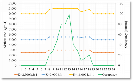
The scheduled airflow rate for a one-day period is shown in
Figure 1. The figure shows a comparison of the airflow profiles (left axis) by employing the three values of K (orange, blue and yellow colored lines, respectively). The airflow rates are related to the nominal airflow rate of the fan Gfan according to Eq. (8) and Eq. (9):
If Gair < 0.2 ∙Gfan : Gair = 0.2 ∙Gfan kg·h-1 (8)
If Gair >Gfan : Gair = Gfan kg·h-1 (9)
Finally, the green colored line shows the daily occupancy profile adopted for each day in the year (right axis).
All simulations are carried out under dynamic conditions by employing a one-hour time step. The analysis is performed by using a simulation time period of one year.
Figure 1. Hourly quasi-constant airflow rate and occupancy profile
In this section, the results of several simulations are presented and carefully discussed. In the first subsection, results obtained by considering a control system based on an adjustable airflow rates are shown. In the second subsection, results related to a control system based on an adjustable inlet temperature of the microclimate environment are analyzed. Finally, a comparison between the two control systems is presented.
4.1 Control system with adjustable airflow rate
The control system with variable airflow rate adjusts the airflow rate based on the required set-point temperature of the moist air in the controlled environment in order to guarantee comfort conditions.
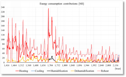
Figure 2. Detailed energy consumptions vs time (March) obtained with AC_Code 2.0 for Potenza, Case A.
As a baseline case, the weather conditions of Potenza and the operating conditions of Case A of Table 2 have been chosen. Taken March as an example, Figure 2 shows the hourly energy consumption versus time in terms of heating/cooling and humidification/dehumidification energy consumptions. The diagram shows also the hourly consumptions due to the reheat process (when it occurs). The figure shows that the cooling energy consumption is equal to the reheat energy (except for a number of hours within the range 1989 ÷2160 h). This is because the cooling contribution is mainly due to the sensible heat removed from the mixture during the dehumidification process. Then, during the reheat process, the same amount of energy previously removed from the airflow rate is provided. In this case, the cooling process occurs only in order to dehumidify the moist air and not to control the temperature of the mixture.
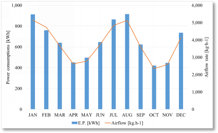
Figure 3 shows on the left axis the monthly electrical power consumptions for a one-year time period obtained with an adjustable airflow rate control system. In the same figure, the required monthly averaged airflow rate is shown on the right axis. January and August are the time periods with the highest electrical power consumption due to the maximum request of airflow rate in winter and summer seasons, respectively.
Finally, Figure 4 summarizes the global energy consumptions in the year. Specifically, red colored columns show the hot water consumptions due to heating, humidification and reheat processes. As expected, significant energy contributions are required on January, February and December, which are the coldest months. On the other hand, on July and August, the highest cooling energy is required although the cooling request is not negligible for the other months of the year. This is due to the relatively low values of the set-point conditions, especially as regards humidity.
Figure 3. Monthly electrical power consumption and monthly average airflow rate (AC_Code 2.0 Potenza, CaseA)
Figure 4. Hot and cold-water consumptions in one-year with AC_Code 2.0 for Potenza, Case A.
In order to analyze the sensitivity to different climatic conditions, three Italian cities are considered, i.e. Turin, Rome and Potenza. Besides, dynamic simulations are carried out under different operating conditions. The results of the analysis are summarized in Figure 5 in terms of hot water consumption, which includes heating, humidification and reheat energy contributions. The hot water consumptions increase/decrease when the set-point thermo-hygrometric parameters increase/decrease. The trend of the hot water consumption with the operating conditions is the same for the three cities, even if the actual consumption depends on the climatic conditions. In fact, Turin and Potenza, due to the cold weather conditions in the winter, need for a higher amount of energy than Rome for the three cases.
Figure 5. Annual hot water consumption for the three cases for Turin, Rome and Potenza with AC_Code 2.0
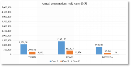
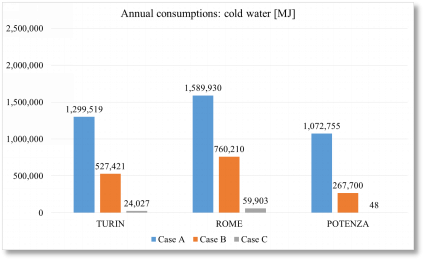
In Figure 6, the cold-water consumption is shown. This amount of energy is due to cooling and dehumidification. Going from Case A to Case C, the cold-water request decreases for all cities because the set-point temperature increases. In all three cases, Rome requires the highest amount of cold water, followed by Turin and then Potenza.
Figure 6. Annual cold-water consumption in the three cases for Turin, Rome and Potenza with AC_Code 2.0
Figure 7. Annual electrical power consumption in the three cases for Turin, Rome and Potenza with AC_Code 2.0
Finally, the electrical power consumption is given in Figure 7.
Such a consumption depends on both climatic conditions and set-point thermo-hygrometric parameters. Case C requires the highest E.P. for all cities because the airflow rate is higher than the other two cases. Going from Case A to Case C, the electrical power consumption increases for the three cities.
4.2 Control system with adjustable inlet temperature
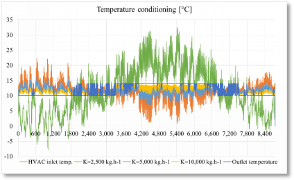
The airflow control system with an adjustable inlet temperature sets the conditioned environment inlet temperature in order to achieve the comfort set-up within the conditioned environment. Three different airflow rates have been chosen in order to analyze the performance of the conditioning system in terms of energy and electrical power consumptions, by setting K to 2,500, 5,000 and 10,000 kgžh-1, respectively. For the city of Potenza under Case A, the control system sets the inlet temperature of the conditioned environment as shown in Figure 8 (2,500 kgžh-1- orange colored line, 5,000 kgžh-1- light blue colored line and 10,000 kgžh-1- yellow colored line). The same figure shows the HVAC inlet temperature (green colored line) and the conditioned environment outlet temperature (blue colored line), which is within the range of comfort. The computed inlet temperature decreases/increases by increasing the airflow rate during the cold/warm season. Therefore, with the same climatic conditions and set-point parameters, higher airflow rates reduce the gap between temperature at the inlet and the outlet of the controlled microclimate.
Figure 8. Inlet temperature by varying the airflow rate with AC_Code 3.0 (Potenza – Case A)
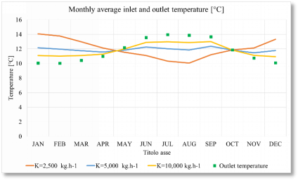
Figure 9. Monthly average inlet and outlet temperature with AC_Code 3.0 (Potenza – Case A)
The monthly average inlet temperature is shown in Figure 9 for all K values together with the outlet temperature. By increasing the airflow rates, the inlet temperature decreases/increases during the cold/warm season, whereas around the end of April and in mid-October the inlet temperatures are almost the same.
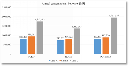
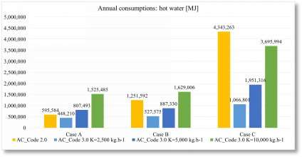
Simulations have been carried out by considering all set-point and weather data conditions for the three airflow rate profiles. In this subsection, for the sake of conciseness, the results related to K equal to 5,000 kgžh-1 are presented. In Figure 10 a comparison in terms of hot water consumption is shown for all cities and set-point conditions. The figure shows that the trend of the hot water consumption is the same as for the case of a control system with adjustable airflow rate (see Figure 5).
Figure 10. Annual hot water consumption for the three cases and cities with AC_Code 3.0 (K =5,000 kgžh-1)
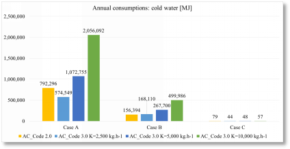
The cold-water consumption is reported in Figure 11. The figure shows that the cold-water demand is higher than the hot water consumption for Case A for all the cities, whereas it is lower for Cases B and C. In agreement with the findings in the previous subsection, the cold-water request decreases when the set-point parameters move from Case A to Case C. Moreover, Figure 11 shows that Rome requires the highest amount of cold water compared to the other cities for the same operating conditions, whereas Potenza requires the lowest cooling/dehumidification energy contribution. A reason could be due to the milder climatic summer conditions of Potenza (in spite of its location in the southern Italy) than Turin.
Figure 11. Annual cold-water consumption for the three cases and cities with AC_Code 3.0 (K =5,000 kgžh-1)
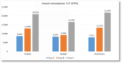
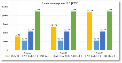
Finally, the electrical power consumption is shown in Figure 12. As expected, the electrical power requirement is the same for all cities and for all climatic conditions because the control system provides a daily airflow rate that does not depend on climatic and operating conditions. By setting K to 2,500, 5,000 and 10,000 kgžh-1 the electrical power consumptions are 5,574, 10,825 and 22,386 kWhžyear-1, respectively.
Figure 12. Annual E.P. consumption for the three cases and cities with AC_Code 3.0 (K =5,000 kgžh-1)
4.3 Comparison between the two control systems
In this subsection, a comparison of the two control systems is carried out to investigate their behavior under different operating conditions. Specifically, the analysis has been carried out by considering the weather data set of Potenza.
Figure and Figure 14 exhibit the request of hot and cold water, respectively. The control system with adjustable inlet temperature and K=2,500 kgžh-1 is the most efficient one, except for the cold-water consumption under operating conditions B, where the control system with adjustable airflow rate gives a somewhat lower consumption.
For both control systems, the hot/cold water consumption increases/decreases moving from Case A to Case C, even if the relative increase/decrease is different for the various cases. For example, the ratio between the hot water consumption of Case C and B is equal to about 3.5 with AC_code 2.0, whereas it is around 1.4 when AC_code 3.0 with K=2,500 kgžh-1 is used.
As regards AC_code 3.0, a reduction of the airflow rate gives lower consumption in terms of both hot and cold water for all operating conditions.
Figure 13. Sensitivity analysis of the control systems: annual hot water consumption for Potenza
Finally, the electrical power consumption is shown in Figure 15.
As regards the control system with adjustable inlet temperature, it has been already pointed out that the electrical consumption does not change with operating conditions. By considering the control system with adjustable airflow rate, the electrical power consumption follows the airflow rate requirement. As expected, the control system with the lowest airflow rate demand, i.e. K=2,500 kgžh-1, is the most efficient.
Figure 14. Sensitivity analysis of the control systems: annual cold-water consumption for Potenza
Figure 15. Sensitivity analysis of the control system: annual electrical power consumption for Potenza
The aim of the present work is the analysis of HVAC control systems to adjust thermo-hygrometric microclimate conditions for a controlled environment. Specifically, the AC_Code model, developed and validated in Ref. [1], has been re-considered and two upgraded versions (AC_Code 2.0 and 3.0) are developed by implementing different control systems. In AC_Code 2.0, a control system with adjustable airflow rate and fixed thermo-hygrometric conditions at the inlet of the controlled environment is implemented, whereas in AC_Code 3.0 a control system with adjustable inlet temperature of the microclimate environment is provided. Several simulations have been carried out in order to analyze the performance and efficiency of HVAC systems in terms of energy requirement with different climatic conditions and different operating conditions. To this end, three Italian cities, Turin, Rome and Potenza have been chosen as different climatic zones and three different temperature and relative humidity comfort ranges are employed, as summarized in Table 2 (Case A, B and C). Moreover, as regards the adjustable inlet temperature control system, scheduled hourly airflow rates for a one-day period have been employed by considering three airflow rates that consist of a constant airflow rate contribution, 2,500 kgžh-1, 5,000 kgžh-1 and 10,000 kgžh-1, respectively, plus a contribution that is a function of the hourly occupancy of the environment.
By considering the weather conditions of Potenza and the operating conditions of Case A (baseline case), the analysis of HVAC system with adjustable airflow rate has shown that January, February and December are the time periods with the highest hot water request. As regards the cold-water requirement, a significant amount of water occurs for the whole year, due to the relatively low values of the set-point parameters employed, especially as regards humidity. The electrical power consumption due to the fan/extractor strictly follows the increase/decrease vs time of the airflow rate. The sensitivity analysis to different climatic and operating conditions shows that the energy consumption of the three cities is characterized by the same trend with the operating conditions, even if the actual consumption depends on climatic conditions. As expected, also the electrical power consumption depends on both climatic conditions and set-point thermo-hygrometric parameters because the control system operates on the airflow rate in order to guarantee the indoor comfort.
For the baseline case, the analysis of HVAC system based on adjustable inlet temperature of the controlled environment has been carried out by employing three values of K (2,500, 5,000 and 10,000 kgžh-1). The computed inlet temperature decreases/increases during the cold/warm season by increasing K. Therefore, with the same climatic conditions and set-point parameters, higher airflow rates reduce the gap between temperature at the inlet and the outlet of the controlled microclimate. Specifically, moving from K equal to 2,500 kgžh-1 to 10,000 kgžh-1, the inlet temperature changes with the seasons and the monthly average values of the three temperatures correspond each other at the end of April and in mid-October, when the change of season occurs.
The results with the control system based on an adjustable inlet temperature and K equal to 5,000 kgžh-1 are given for the three cities and the three different set-up conditions. The energy consumption with different operating conditions follows the same trend as for the other control system. The results in terms of cold water show that the cold-water demand is higher than the hot water consumption for Case A and for all cities, whereas it is lower for Case B and even lower for Case C. The city of Rome needs for the highest energy requirement compared to the other two cities for the same operating conditions, whereas the city of Potenza is characterized by the lowest cooling/dehumidification energy request. The electrical power requirement is the same for all cities and set-up because the control system is based on an adjustable inlet temperature that does not depend on climatic and operating conditions.
Finally, a comparison between the two control systems has been carried out by employing Potenza weather conditions. The system based on an adjustable inlet temperature with the lowest value of K provides the best control system for all cases, in terms of both energy and electrical power consumption. The only exception is the cold-water consumption for case B, where the regulation with adjustable airflow rate gives a somewhat lower consumption.
|
T |
Temperature, °C |
|
tol |
Tolerance |
|
E.P. |
Electrical Power, kW |
|
G P |
Airflow rate, kgžh-1 Nominal electrical power, kW |
|
Q |
External airflow rate to number of person, litersžs-1žperson-1 |
|
K |
Constant airflow rate, kgžh-1 |
|
Greek symbols |
|
|
$\rho $ |
Air density, kgžm-3 |
|
$\beta$ |
User constant, [-]
|
|
Subscripts |
|
|
out |
outlet conditions |
|
ext |
external conditions |
|
setpoint |
set-point parameter |
|
T |
temperature |
|
air |
related to airflow |
|
fan |
related to fan device |
|
ext |
related to extractor device |
|
breakt |
air breakthrough |
|
op |
per person |
[1] Genco A., Viggiano A., Viscido L., Sellitto G., Magi V. (2016). Numerical simulation of energy systems to control environment microclimate, Int J Heat & Tech, Vol. 34, No. Special Issue 2, pp. S545-S552. DOI: 10.18280/ijht.34Sp0249
[2] University of Wisconsin, Madison. Energy Simulation Software, from http://sel.me.wisc.edu/trnsys/index.html
[3] Nik V.M., Mata E., Kalagasidis A.S. (2015). Assessing the efficiency and robustness of the retrofitted building envelope against climate change, Energy Procedia, Vol. 78, pp. 955-960. DOI: 10.1016/j.egypro.2015.11.031
[4] Genco A., Viggiano A., Rospi G., Cardinale N., Magi V. (2015). Dynamic modeling and simulation of buildings energy performance based on different climatic conditions, Int J Heat & Tech, Vol. 33, No. 4, pp. 107-116. DOI: 10.18280/ijht.330414
[5] Scardigno D., Fanelli E., Viggiano A., Braccio G., Magi V. (2015). A genetic optimization of a hybrid organic Rankine plant for solar and low-grade, energy sources, Energy, Vol. 91, pp. 807-815. DOI: 10.1016/j.energy.2015.08.066
[6] Fadaee M., Radzi M.A.M. (2012). Multi-objective optimization of a stand-alone hybrid renewable energy system by using evolutionary algorithms: A review, Renewable and Sustainable Energy Reviews, Vol. 16, No. 5, pp. 3364-3369. DOI: 10.1016/j.rser.2012.02.071
[7] Mathews E.H., Botha C.P., Arndt D.C., Malan A. (2001). HVAC control strategies to enhance comfort and minimise energy usage, Energy and Buildings, Vol. 33, No. 8, pp. 853-863. DOI: 10.1016/S0378-7788(01)00075-5
[8] Congradac V., Kulic F. (2009). HVAC system optimization with CO2 concentration control using genetic algorithms, Energy and Buildings, Vol. 41, No. 5, pp. 571-577. DOI: 10.1016/j.enbuild.2008.12.004
[9] Fong K.F., Hanby V.I., Chow T.T. (2006, Mar.). HVAC system optimization for energy management by evolutionary programming, Energy and Buildings, Vol. 38, No. 3), pp. 220-231. DOI: 10.1016/j.enbuild.2008.12.004
[10] Fong K.F., Hanby V.I., Chow T.T. (2009). System optimization for HVAC energy management using the robust evolutionary algorithm, Applied Thermal Engineering, Vol. 29, No. 11-12, pp. 2327-2334. DOI: 10.1016/j.applthermaleng.2008.11.019
[11] EnergyPlus. Energy Simulation Software, from https://energyplus.net/weather region/europe_wmo_region_6/ITA%20%20
[12] UNI 10339:1995–Impianti aeraulici al fine di benessere, Generalità, classificazione e requisiti, Regole per la richiesta d'offerta, l'offerta, l'ordine e la fornitura.