OPEN ACCESS
In this work a simple predictive model to estimate PV/T collector performance is presented. The model is based on an equivalent electrical circuit of the collector, whose solution allows evaluation of its thermal and electrical power produced. The electrical circuit is modified according to whether the problem is solved in stationary or transient conditions. As regards the stationary approach, two different circuits can be schematized: the first allows evaluation of the magnitudes at different points along the motion direction of the fluid; the resolution of the second electric circuit allows direct evaluation of the average magnitudes between the inlet and outlet collector section. With the transient model, instead, it is possible to estimate the behaviour of the collector by adding, to the previous circuit, a capacitor of capacity equal to those of the thermal collector. Obviously, when the transient condition is exhausted, the various determined quantities are identical to those measured in stationary conditions. Finally, the study shows that the electrical circuit used for this type of collector is similar to that of the solar thermal collector, with the difference that some circuit components also contain electrical quantities.
electrical analogy, solar collectors, PV/T collectors
Among the various sources of energy, certainly, solar energy has a basic role in meeting global energy needs and in the air pollution reduction [1]. The solar energy is collected by means of photovoltaic and thermal panels. The photovoltaic panels convert solar energy directly into electricity, while the thermal panels (or collectors) convert it into thermal energy of a heat transfer fluid.
PV/T cogenerative technology, the subject of research and development since the ’70s, arises from the need to improve the low efficiency of the PV system and also, using the heat generated as a product, to provide easily both electricity and heat. Therefore, they can replace cogeneration plants which use non-renewable resources [2]. PV/T collectors are simple to incorporate in the facades or on the roofs of buildings and therefore they are suitable to real applications. One of the main advantages of the PV/T technology is the fact that the collection surface used is roughly halved for the same electrical and heat products, when compared with that required by separated panels (PV and thermal). This aspect is more evident especially when the surface has significant sizes [3].
The aim of the present work is to identify simple alternative methodologies, to allow the estimation of the cogenerative solar collectors performance. This is possible using electrical analogy. Two systems are similar when they are governed by similar equations and have similar conditions to the limit: the equation that describes the behavior of a system can be transformed into the equation of the other system simply by changing the variable symbols. For example, thermal conduction in solids is, in many ways, similar to electrical conduction in the conductors. Therefore, a thermal circuit corresponds to each electrical circuit and vice versa. Specifically, the thermal parameters such as power, temperature and heat capacity, are equivalent, respectively, to the following electrical parameters: current, voltage and capacity.
In this case, the equivalent electric circuit of the collector allows resolution of the power balance. The various terms in the equation are combined to circuit elements; for example, the power absorbed by the collector is represented by means of a current generator, while the external air temperature by means of a voltage generator. In addition, the electric circuit is suitably modified as a function of the system conditions: stationary or transient.
In this work it is shown that the circuit relating to the solar thermal collector can also be used for the PV/T collector, through the redefinition of certain circuit magnitudes so as to take account also of the electrical component.
The instantaneous heat balance equation of a solar collector, with reference to the power absorbed by the plate, is:
$G_{c} A_{c}(\tau \alpha)=Q_{u}+Q_{p}+\frac{d U_{p}}{d t}$ (1)
where Gc is the global radiation incident on the collector plane, Ac is the absorbing surface area, (τα) is the effective product between the cover transmission coefficient and the plate absorption coefficient, Qu is the thermal power given to the heat transfer fluid, Qp is the power lost by radiation and convection, while $\frac{d U_{p}}{d t}$ is the power accumulated by the plate.
2.1 Stationary thermal analysis
Setting the solar irradiance absorbed with S [S=Gc·(τα)], the plate temperature with Tp and the fluid temperature with Tf, Eq. (1), written in stationary conditions, for an element of area (W·dx), becomes:
$S=\frac{\dot{m} c_{p}}{W} \frac{d T_{f}(x)}{d x}+\frac{\left(T_{p}(x)-T_{a}\right)}{\frac{1}{U_{c}}}=C_{f} \frac{d T_{f}(x)}{d x}+\frac{\left(T_{p}(x)-T_{a}\right)}{R_{e}}$ (2)
where Cf is the hourly specific thermal capacity of the fluid, W is the collector width, Uc is the global heat exchange coefficient between plate and external air and Ta is the external air temperature.
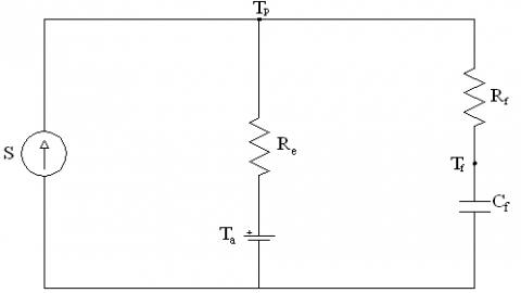
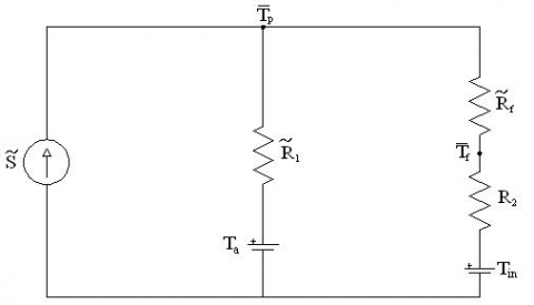
Referring to Eq. (2) it is possible to schematize the equivalent electric circuit shown in Figure 1.
Figure 1. Equivalent electric circuit
In the electric circuit shown in Figure 1, Re represents the thermal resistance between the plate and the external air (equal to 1/Uc) and Rf is the thermal resistance between the plate and the fluid. The latter is obtained as the difference between the fluid-external air resistance and the plane-external air resistance:
$R_{f}=\frac{1}{F^{\prime} U_{c}}-\frac{1}{U_{c}}$
The use of a capacitive element is not related to the transient modeling of the solar collector. In fact, for the stationary analysis, the capacitor is simply used as an integral element in the circuit and the time is simply analogous to the distance [4].
The resolution of this circuit allows the temperature of the plate and that of the heat transfer fluid to be estimated and, therefore, the thermal power transferred to the fluid at different points, along the fluid motion direction (from the collector inlet section x = 0 to collector outlet section x = L).
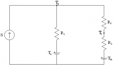
Since, to estimate the average useful power between inlet and outlet it is necessary to solve the circuit and then calculate the mean arithmetic value between the magnitudes evaluated in the two extreme sections, it was considered appropriate to schematize a second electrical circuit in which the magnitudes estimated are already averages, so as to make the immediate calculation. With the new circuit the analysis can be extended to more irradiation values (time values) on the plane of the collector and, therefore, to perform the estimation of the useful daily power.
The electrical circuit of Figure 2, in this case, describes the following thermal balance:
$S=\frac{\left(\overline{T}_{f}-T_{i n}\right)}{\frac{A_{c}}{2 \dot{m} c_{p}}}+\frac{\left(\overline{T}_{p}-T_{a}\right)}{\frac{1}{U_{c}}}=\frac{\left(\overline{T}_{f}-T_{i n}\right)}{R_{2}}+\frac{\left(\overline{T}_{p}-T_{a}\right)}{R_{1}}$ (3)
with the hypothesis:
$\overline{T}_{f}=\frac{T_{o u t}+T_{i n}}{2}$
where Tin and Tout represent, respectively, the inlet and outlet temperature of the fluid.
Figure 2. Equivalent electric circuit, average magnitudes
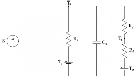
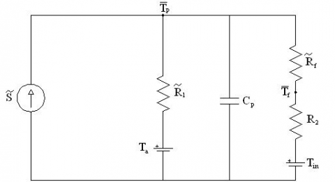
Figure 3. Equivalent electric circuit in transient conditions
2.2 Transient thermal analysis
Eq. (3), written in transient conditions, becomes:
$S=\frac{\left(\overline{T}_{f}-T_{i n}\right)}{R_{2}}+\frac{\left(\overline{T}_{p}-T_{a}\right)}{R_{1}}+(m c)_{p} \frac{d \overline{T}_{p}}{d t}$ (4)
where (mc)p represents the heat capacity (specific) of the plate Cp [J. m-2. K-1].
The electric circuit, that describes Eq. (4), is schematized in Figure 3.
Hybrid thermal-photovoltaic solar collectors [3], or PV/T, are systems able to convert simultaneously solar energy into electricity and heat. A PV/T collector, generally, is composed of a coil, or of a bundle of tubes in parallel, in which the heat transfer fluid circulates and above which the photovoltaic module is glued, by means of a highly conductive glue, or laminated; they can be glazed or uncovered. Figure 4 shows an assembly drawing of a PV/T glazed collector.
Figure 4. Assembly drawing of a PV/T collector [3]
The instantaneous heat balance equation of the absorber plate, in the case of the PV/T collector, is described by Eq. (5).
$G_{c}(\tau \alpha) A_{c}=\tilde{Q}_{u}+Q_{p}+Q_{e}+\frac{d U_{p}}{d t}$ (5)
where, the useful power transferred to the heat transfer fluid is indicated with $\tilde{\mathrm{Q}}_{\mathrm{u}}$ while Qe represents the useful electrical power generated.
3.1 Stationary thermal analysis
The specific electrical power is calculated by the following expression:
$q_{e}=\frac{Q_{e}}{A_{c}}=\eta_{e} G_{c}$ (6)
where, ηe represents the electrical efficiency [5]:
$\eta_{e}=\eta_{R}\left[1-\beta\left(T_{c}-\mathrm{T}_{R}\right)+\gamma \log _{10} G_{c}\right]$ (7)
Given the hypothesis that the plate temperature is coincident with the photovoltaic laminate temperature Tc = Tp, Eq. (5), written in stationary conditions, for an element of area (W·dx), becomes:
$G_{c}(\tau \alpha)=\frac{\dot{m} c_{p}}{W} \frac{d T_{f}(x)}{d x}+U_{c}\left(T_{p}(x)-T_{a}\right)+\eta_{R}\left[1-\beta\left(T_{p}(x)-T_{R}\right)+\gamma \log _{10} G_{c}\right] G_{c}$ (8)
With simple algebra [3, 6], Eq. (8) can be rewritten as:
$G_{c}(\tau \alpha)\left(1-\frac{\eta_{R}\left[1-\beta\left(T_{a}-T_{R}\right)+\gamma \log _{10} G_{c}\right]}{(\tau \alpha)}\right)=C_{f} \frac{d T_{f}(x)}{d x}+\left(T_{p}(x)-T_{a}\right) \cdot\left(U_{c}-\eta_{R} \beta G_{c}\right)$ (9)
Setting:
$\tilde{S}=G_{c}(\tau \alpha)\left(1-\frac{\eta_{R}\left[1-\beta\left(T_{a}-T_{R}\right)+\gamma \log _{10} G_{c}\right]}{(\tau \alpha)}\right)=G_{c}(\tau \alpha)\left(1-\frac{\eta_{a}}{(\tau \alpha)}\right)=S \cdot\left(1-\frac{\eta_{a}}{(\tau \alpha)}\right)$ (10)
$\tilde{U}_{c}=U_{c}-\eta_{R} \beta G_{c}=U_{c}-\frac{S}{(\tau \alpha)} \eta_{R} \beta$ (11)
where ha is the electrical efficiency of the collector when the cell temperature is equal to external air temperature.
Eq. (9) becomes:
$\tilde{S}=C_{f} \frac{d T_{f}(x)}{d x}+\frac{\left(T_{p}(x)-T_{a}\right)}{\frac{1}{\hat{U}_{c}}}=C_{f} \frac{d T_{f}(x)}{d x}+\frac{\left(T_{p}(x)-T_{a}\right)}{\tilde{R}_{e}}$ (12)
This last expression, with the change of variables introduced, is identical to Eq. (2) relative to the traditional thermal collector.
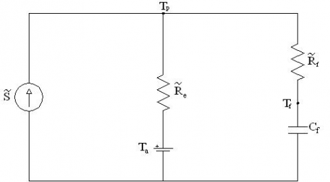
Referring to Eq. (12) it is possible to schematize the equivalent electric circuit shown in Figure 5.
The electrical circuit of Figure 5 is similar to that of Figure 1, with the difference that some circuit variables also contain the electrical component in accordance with Eqs. (10) and (11).
Figure 5. Equivalent electric circuit, PV/T collector
Using Eqs. (13) and (14), which describe the specific useful power, and Eq. (12), a differential equation of the first order is obtained; the resolution of this equation allows the expression for the calculation of the local fluid temperature to be obtained and, therefore, that for the calculation of the local plate temperature, along the fluid motion direction.
$q_{u}(x)=C_{f} \frac{d T_{f}(x)}{d x}$ (13)
$q_{u}(x)=\frac{T_{p}(x)-T_{f}(x)}{\tilde{R}_{f}}$ (14)
$T_{f}(x)=T_{i n}+T^{\prime} \cdot\left(1-e^{-\frac{x}{R C_{f}}}\right)$ (15)
$T_{p}(x)=T_{i n}+T^{\prime} \cdot\left(1-\frac{\tilde{R}_{e}}{R} e^{-\frac{x}{R C_{f}}}\right)$ (16)
where:
$T^{\prime}=\left(T_{a}-T_{i n}+\tilde{S} \tilde{R}_{e}\right)$
$R=\tilde{R}_{e}+\tilde{R}_{f}$
Integrating Eqs. (15) and (16) over the entire length of the plate, the equations for the calculation of the plate and fluid average temperature and, therefore, the equations to calculate the thermal and electrical average powers are obtained:
$\overline{q}_{u}=\tilde{F}_{R}\left(\tilde{S}-\tilde{U}_{c}\left(T_{i n}-T_{a}\right)\right)$ (17)
$\overline{q}_{e}=\eta_{a} G_{c}-\eta_{R} \beta G_{c}\left(\frac{\tilde{S}}{\tilde{U}_{c}}\left(1-\tilde{F}_{R}\right)+\left(T_{i n}-T_{a}\right) \tilde{F}_{R}\right)$ (18)
Also for the PV/T collector, as for the traditional thermal collector, it is appropriate to schematize a second electric circuit as a function of the average quantities rather than local ones. In this case the electric circuit (Figure 6) describes the following thermal balance:
$\tilde{S}=\frac{\left(\overline{T}_{f}-T_{m}\right)}{\frac{A_{c}}{2 \dot{m} c_{p}}}+\frac{\left(\overline{T}_{p}-T_{a}\right)}{\frac{1}{\tilde{U}_{c}}}=\frac{\left(\overline{T}_{f}-T_{m}\right)}{R_{2}}+\frac{\left(\overline{T}_{p}-T_{a}\right)}{\tilde{R}_{1}}$ (19)
Figure 6. Equivalent electric circuit (average magnitudes), PV/T collector
Taking into account the change of variables, Eqs. (10) and (11), the electrical circuit of Figure 6, relative to the PV/T collector, is similar to that of Figure 2 corresponding to the traditional thermal collector.
3.2 Transient thermal analysis
Eq. (19), written in transient conditions, becomes:
$\tilde{S}=\frac{\left(\overline{T}_{f}-T_{i n}\right)}{R_{2}}+\frac{\left(\overline{T}_{p}-T_{a}\right)}{\tilde{R}_{1}}+(m c)_{p} \frac{d \overline{T}_{p}}{d t}$ (20)
The circuit that describes Eq. (20) is shown in Figure 7; also in this case, the electric circuit is similar to that of Figure 3 relative to the traditional thermal collector.
Figure 7. Equivalent electric circuit in transient conditions, PV/T collector
To verify the correctness of the results provided by the models, initially a solar thermal collector, whose characteristics are summarized in Table 1, is used. In the same table, also the data of solar radiation on the collector plane, external air temperature and temperature of the incoming fluid to the collector are reported.
Table 1. Input data for the analysis
|
Absorbing surface area Ac [m2] |
1.91 |
|
Mass flow rate of the fluid [kg/s] |
0.01592 |
|
Transmittance |
0.91 |
|
Absorbance |
0.95 |
|
Zero loss efficiency η0 [%] |
78.5 |
|
First order heat loss coefficient a1 [W/m2K] |
3.722 |
|
Second order heat loss coefficient a2 [W/m2K2] |
0.012 |
|
Thermal capacity Cp [J/m2K] |
9543 |
|
Global radiation Gc [W/m2] |
800 |
|
External air temperature Ta [°C] |
23 |
|
Fluid temperature in the inlet section Tfi [°C] |
30 |
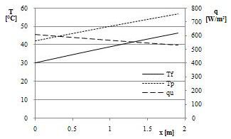
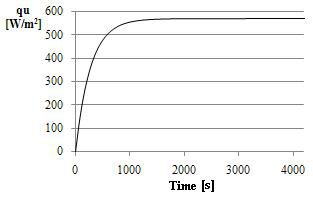
By the resolution of the circuit shown in Figure 1, the local values of the plate temperature Tp, of the fluid temperature Tf and of the specific useful power qu, along the motion direction, are obtained; their trend is shown in Figure 8. The average value of the specific useful power obtained is of 568 W/m2. By the resolution of the circuit shown in Figure 2 (stationary conditions and average magnitudes), instead, a value of the specific useful power of 568.8 W/m2 is obtained. The same value, as shown in Figure 9, is reached asymptotically with the resolution of the electric circuit in transient conditions (Figure 3), when the transient condition is exhausted.
Figure 8. Fluid temperature, plate temperature and specific useful power trend
Figure 9. Specific useful power trend in transient conditions
In Figure 10, the comparison between the power curve obtained by resolution of the circuit under transient conditions and the power curve given by the collector manufacturer is shown. The comparison is made for a constant solar irradiation value of 1000 W/m2. The same results are presented in Table 2, in which also the percentage error between the two solutions is estimated:
$\varepsilon=\frac{Q_{\text {ucalc}}-Q_{\text {ureal}}}{Q_{\text {ural}}} \%$ (21)
The small difference between the two solutions is attributable to the evaluation of a single value of the global heat exchange coefficient Uc, non provided by the manufacturer. It is derived from coefficients a1 and a2.
For the analysis of the models relative to the PV/T collector, a collector with the characteristics reported in Table 3 is used.
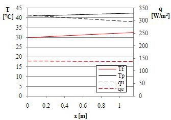
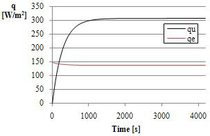
By the resolution of the circuit shown in Figure 5, the local values of the plate temperature Tp, of the fluid temperature Tf and of the thermal and electrical specific useful power (qu and qe), along the motion direction, are obtained; their trend is shown in Figure 11. The average values of these quantities are, respectively, equal to 41.74 °C, 31.29 °C, 308.7 W/m2 and 139 W/m2. By the resolution of the circuit shown in Figure 6, the following results are obtained: $\overline{\mathrm{T}}_{\mathrm{p}}$ = 41.73 °C, $\overline{\mathrm{T}}_{\mathrm{f}}$ = 31.27 °C, $\overline{\mathrm{q}}_{\mathrm{u}}$ = 308.9 W/m2 e $\overline{\mathrm{q}}_{\mathrm{e}}$ = 139 W/m2. The same values of the thermal and electrical power, as shown in Figure 12, are reached asymptotically with the resolution of the electric circuit in transient conditions (Figure 7), when the transient condition is exhausted.
Figure 10. Real and calculated power curve
Table 2. Real and calculated power
|
$\overline{\mathrm{T}}_{\mathrm{f}}$ -Ta [°C] |
QuReal [W] |
QuCalc [W] |
ε [%] |
|
0 |
1499.35 |
1536.02 |
2 |
|
10 |
1425.97 |
1442.01 |
1 |
|
20 |
1348.00 |
1348.00 |
0 |
|
30 |
1265.45 |
1253.99 |
-1 |
|
40 |
1178.32 |
1159.98 |
-2 |
|
50 |
1086.60 |
1065.97 |
-2 |
|
60 |
990.30 |
971.96 |
-2 |
|
70 |
889.41 |
877.95 |
-1 |
|
80 |
783.94 |
783.94 |
0 |
|
90 |
673.89 |
689.93 |
2 |
|
100 |
559.25 |
595.92 |
7 |
Table 3. Input data for the PV/T collector
|
Absorbing surface area Ac [m2] |
1.15 |
|
Mass flow rate of the fluid [kg/s] |
0.033333 |
|
Zero loss efficiency η0 [%] |
55 |
|
First order heat loss coefficient a1 [W/m2K] |
6.3 |
|
Second order heat loss coefficient a2 [W/m2K2] |
0.08 |
|
Thermal capacity Cp [J/m2K] |
11478.26 |
|
Temperature coefficient for cell efficiency β [°C-1] |
0.0045 |
|
Rated voltage Vmp [V] |
30.5 |
|
Rated current Imp [A] |
8.2 |
|
Global radiance Gc [W/m2] |
800 |
|
External air temperature Ta [°C] |
25 |
|
Fluid temperature in the inlet section Tfi [°C] |
30 |
Figure 11. Fluid temperature, plate temperature, specific thermal and electrical power trend, PV/T collector
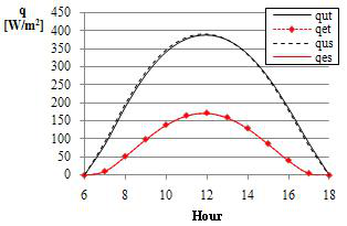
Finally, the hourly values of thermal and electrical power have been determined for the PV/T collector for a whole day in stationary and transient conditions.
The results obtained are presented in Table 4 and shown in Figure 13.
Figure 12. Specific thermal and electrical power trend in transient conditions, PV/T collector
Table 4. Comparison of thermal and electrical power estimated with the stationary and transient model, for a PV/T solar collector
|
Hour |
Ta |
Gc |
qus |
qes |
qut |
qet |
|
[°C] |
[W/m2] |
[W/m2] |
[W/m2] |
[W/m2] |
[W/m2] |
|
|
6 |
24.3 |
69.79 |
0 |
0 |
0 |
0 |
|
7 |
25.46 |
257.59 |
91.6 |
10.98 |
84.16 |
11.05 |
|
8 |
26.94 |
466.14 |
196.62 |
52 |
188.86 |
52.14 |
|
9 |
28.06 |
656.89 |
284.58 |
98.8 |
277.97 |
98.96 |
|
10 |
28.58 |
803.36 |
346.19 |
138.85 |
341.51 |
138.99 |
|
11 |
28.7 |
892.28 |
380.77 |
164.57 |
378.12 |
164.66 |
|
12 |
28.7 |
916.57 |
389.79 |
171.77 |
389.10 |
171.79 |
|
13 |
28.7 |
875.06 |
374.35 |
159.51 |
375.55 |
159.47 |
|
14 |
28.58 |
770.87 |
333.84 |
129.68 |
336.98 |
129.59 |
|
15 |
28.12 |
612.94 |
267.87 |
87.36 |
273.00 |
87.24 |
|
16 |
27.26 |
419.15 |
180.17 |
41.55 |
187.03 |
41.44 |
|
17 |
26.18 |
221.96 |
82.33 |
5.48 |
90.06 |
5.42 |
|
18 |
25.14 |
66.78 |
0 |
0 |
1.28 |
0 |
|
Average [W/m2] |
225.24 |
81.58 |
224.89 |
81.60 |
||
From the results presented in Table 4, it is observed that, under transient conditions, for the capacitive effects of the collector, in the early hours of the day during which the collector is heated, the specific useful power transferred to the heat transfer fluid is less than that obtained under stationary conditions. On the contrary, in the afternoon hours, during which the collector cools down, the specific useful power transferred to the heat transfer fluid is greater than that obtained in stationary conditions (the collector takes more time to cool down).
Figure 13. Thermal and electrical power trend, stationary and transient circuit model, PV/T collector
In this paper a simple predictive model to estimate PV/T collector performance has been presented. The model is based on an equivalent electrical circuit of the collector, whose solution allows the evaluation of thermal and electrical power produced. The electrical circuit is modified according to whether the problem is solved in stationary or transient conditions. As regards the stationary approach, two different circuits were schematized: the first allowed evaluation of the quantities at different points along the motion direction of the fluid; the resolution of the second electric circuit allowed direct evaluation of the average magnitudes between the inlet and outlet collector section. With the transient model, instead, it was possible to estimate the behaviour of the collector by adding a capacitor of capacitance equal to those of the thermal collector to the previous circuit. Obviously, when the transient condition is exhausted, the various determined quantities are identical to those measured in stationary conditions. Finally, the study showed that the electrical circuit used for this type of collector is similar to that of the solar thermal collector, with the difference that some circuit components also contain electrical quantities.
Simulating the behaviour of a thermal solar collector and a cogenerative PV/T solar collector, it was verified that the three circuit models, stationary with local magnitudes, stationary with average magnitudes and transient (when transient is exhausted), provide the same results.
Comparing, instead, the PV/T collector behaviour in stationary and transient conditions, for a whole day, it was observed that, for the capacitive effects of the collector, during the morning hours in which the collector heats, the transient model provides useful power values lower than the stationary model and the opposite in the afternoon hours, during which the collector cools.
|
Ac |
absorbing surface area, m2 |
|
Cf |
hourly specific thermal capacity of the fluid, W. m-1. K-1 |
|
Cp |
plate specific thermal capacity, J. m-2. K-1 |
|
cp |
specific heat of the fluid, J. kg-1. K-1 |
|
F’ |
collector efficiency factor |
|
$\tilde{\mathrm{F}}^{\prime}$ |
PV/T collector efficiency factor |
|
$\tilde{\mathrm{F}}_{\mathrm{R}}$ |
PV/T collector removal factor |
|
Gc |
global radiation on the collector plane, W. m-2 |
|
L |
collector length, m |
|
$\dot{\mathrm{m}}$ |
mass flow rate of the fluid, kg. s-1 |
|
Q |
power, W |
|
$\tilde{\mathrm{Q}}$ |
PV/T power, W |
|
q |
specific power, W. m-2 |
|
$\overline{q}$ |
average specific power, W. m-2 |
|
Re |
thermal resistance between plate and external air for thermal collector, m2. K. W-1 |
|
$\tilde{\mathrm{R}}_{\mathrm{e}}$ |
thermal resistance between plate and external air for PV/T collector, m2. K. W-1 |
|
Rf |
thermal resistance between plate and fluid for thermal collector, m2. K. W-1 |
|
$\tilde{\mathrm{R}}_{\mathrm{f}}$ |
thermal resistance between plate and fluid for PV/T collector, m2. K. W-1 |
|
S |
solar irradiance absorbed by the thermal collector plate W. m-2 |
|
$\tilde{\mathrm{S}}$ |
solar irradiance absorbed by the PV/T collector plate W. m-2 |
|
T |
temperature, °C |
|
$\overline{\mathrm{T}}$ |
average temperature, °C |
|
Uc |
global heat exchange coefficient between plate and external air for a thermal collector, W. m-2. K-1 |
|
$\tilde{\mathrm{U}}_{\mathrm{c}}$ |
global heat exchange coefficient between plate and external air for a PV/T collector, W. m-2. K-1 |
|
Up |
internal energy, J |
|
W |
collector width, m |
|
x |
motion direction of the fluid, m |
|
Greek symbols |
|
|
β |
temperature coefficient for cell efficiency, °C-1 |
|
g |
intensity coefficient for cell efficiency |
|
ε |
percentage error, % |
|
η |
efficiency |
|
ηa |
electrical efficiency with Tc=Ta condition |
|
(τα) |
effective product between the cover transmission coefficient and the plate absorption coefficient |
|
Subscripts |
|
|
a |
external air |
|
c |
cell |
|
e |
electric |
|
es |
electric steady |
|
et |
electric transient |
|
f |
fluid |
|
in |
inlet section |
|
out |
outlet section |
|
p |
plate (collector) |
|
R |
reference conditions |
|
u |
thermal |
|
uCalc |
thermal calculated |
|
uReal |
thermal real |
|
us |
thermal steady |
|
ut |
thermal transient |
[1] Cannistraro A., Cannistraro G., Cannistraro M., Galvagno A. (2016). Analysis of the air pollution in the Urban center of four Sicilian cities, International Journal of Heat and Technology, Vol. 34, Sp. 2, pp. S219-S225. DOI: 10.18280/ijht.34S205
[2] Cannistraro A., Cannistraro G., Cannistraro M., Galvagno A., Trovato G. (2016). Technical and economic evaluations about the integration of cotrigeneration systems in the dairy industry, International Journal of Heat and Technology, Vol. 34, Sp. 2, pp. S332-S336. DOI: 10.18280/ijht.34S220
[3] Cucumo M., Cucumo D., De Rosa A., Ferraro V., Kaliakatsos D., Marinelli V. (2009). Analisi teorica di un collettore solare cogenerativo PV/T a liquido, presented at the Conf. 64° Congresso Nazionale ATI, L’Aquila, Italia.
[4] Sproul A.B., Bilbao J.I., Bambrook S.M. (2012). A novel thermal circuit analysis of solar thermal collectors, 50th Annual Conference, Australian Solar Energy Society (Australian Solar Council), Melbourne, Australia. ISBN: 978-0-646-90071-1.
[5] Evans D.L (1981). Simplified method for predicting photovoltaic array output, Solar Energy, Vol. 27, pp. 555-560. DOI: 10.1016/0038-092X(81)90051-7
[6] Florschuetz L.W. (1979). Extension of the Hottel–Whillier model to the analysis of combined photovoltaic/thermal flat plate collectors, Solar Energy, Vol. 22, pp. 361-366. DOI: 10.1016/0038-092X(79)90190-7