OPEN ACCESS
To prevent a ball becoming stuck in coiled tubing, it is critical to determine the flow velocity of fluid in a hydraulic drive ball-off. The computational fluid dynamics method and standard k-ε turbulence model were applied to simulate the flow within the tubing of a section of coiling block. By analyzing the flow around the ball, the force on the ball exerted by fluid was computed, and the movement trend of the ball at different locations obtained by steady simulation. With the dynamic grid technique, the movement of the ball was identified through transient simulation. The research showed that: the fluid force through static simulation is too large to be used for judging the ball’s passing capacity in a section of coiling block. The ball moved around the coiling block with a minimum value of θ = 90°, revealing that the ball could easily reach the highest point if the minimal angular velocity of ball was greater than zero. Moreover, the conclusion that the ball could pass through the whole section of the coiling block if only it passed the first circle of the coil could be drawn. Furthermore, the critical flow velocity for different sized ball to pass through the coiled tubing increased monotonically with the increase in the ball diameter, and exhibited an approximate quadratic relation. When the curvature radius of the coiling block was 1.268 m and the diameter of the solid steel ball was in the range of (30 mm, 50 mm), the critical flow velocity was (2.30 m/s, 2.415 m/s). This study provides a useful basis for experiment design.
Coiled tubing, Ball-off,Stuck, Passing capacity, Numerical simulation.
Coiled tubing is a long oil pipe wound by a coiling block for entering into and lifting in a well without a threaded connection, and it has been widely applied in drilling, well completion, well logging, oil-gas exploitation and well repair and similar fields, due to the prominent advantages of having a compact structure, convenience of operation, high efficiency, low cost, reservoir protection and increased production [1-2]. Nevertheless, there are still some issues during the operation of coiled tubing, such as the passing capacity of a ball for staged fracturing. As a ball, entering from one open end of the tubing, must pass through the tubing wrapped around the coiling block to reach the wellhead and wellhole, it can become vulnerable to being stuck inside the tubing. Currently, the method of increasing the pressure head is usually adopted to enhance the driving force of the fluid flow. Unfortunately, the risk of the tubing rupturing increases as a result of raising the pressure in the tubing. Obviously, the condition that the ball can pass smoothly through the coiled tubing urgently needs to be determined for the scientific design of the hydraulic drive technology and tubing safety.
In order to obtain the rule for the movement of a ball, it is critical to determine the force acting on the ball [3-4]. H. XIAO et al. [5] analyzed the forces of the ball in vertical wells to deduce the motion equations of the ball in the fracturing fluid, in which the average velocity of pipe flow instead of the actual fluid velocity was used in their hydraulic formula. By solving the equations with the four order Runge-Kutta method, they argued that the ball rapidly entered into a state of steady settlement after it was accelerated rapidly at an initial stage. Other research reported on the dynamic carrying regularity of sand particles in mud, based on a cuttings motion equation and cuttings bed height prediction model [6-7], and the critical return velocity of annulus drilling fluid for safe drilling was identified through a theoretical and numerical method. It is noted that the accuracy of calculation mainly depends on determining the liquid forces acting on the particles, and numerically simulating the flow around the ball. The aim of this study is to simulate the inner flow in tubing wrapped around a coiling block with a steady and transient method, and to analyze the motion rule to identify the possibilities of the ball. This research is useful for the successful operation of coiled tubing.
Assuming that the ball is in coiled tubing wrapped around a coiling block without contacting the internal wall of the tubing, thus the total force $\sum \vec{F}_{m}$ on the ball is
$\sum \vec{F}_{m}=\vec{F}_{G}+\vec{F}_{P}+\vec{F}_{D}+\vec{F}_{A}+\vec{F}_{B}$ (1)
where $\vec{F}_{G}$ is the gravity, N; $\vec{F}_{D}$ is the drag force arising from the fluid shear effect on the ball surface along the flow direction, N [8]; $\vec{F}_{A}$ is the additional mass force [9] created by the acceleration motion of the surrounding fluid driven by the acceleration of the ball, N; $\vec{F}_{B}$ is the hydrodynamic force (Basset force) [10] caused by the boundary layer development lag when the velocity of ball is changed, N; $\vec{F}_{P}$ is the force caused by pressure’s uneven distribution on the surface of the ball, and
$\vec{F}_{P}=\vec{F}_{P 1}+\vec{F}_{P 2}$ (2)
Here, $\vec{F}_{P 1}$ is the pressure gradient force caused by the gravitational field and hydraulic losses on the direction of the flow vector, N; $\vec{F}_{P 2}$ is the lifting force along the radial direction caused by different circulation flow velocity on the both sides of the ball, N.
So the ball movement equation can be described as
$\sum \vec{F}_{m}=m \dot{\vec{v}}_{\text {ball}}$ (3)
As these forces do not point to the gravity center of the ball, a moment is generated around the ball center to make it rotate. If the plane of symmetry is XOY plane, the moment of momentum equation can be expressed as:
$J_{z} \dot{\omega}_{z \mathrm{c}}=\sum M_{z c}\left(\vec{F}_{m}\right)$ (4)
where m is the mass of the ball, kg; \vec{v}_{\text {ball}} is the linear velocity of the ball, m/s; \vec{F}_{m} is the resultant external force applied to the ball, N; Jz is the moment of inertia of the ball on the axis which lies across the center of gravity and parallel to the Z axis, kg·m2; \dot{\omega}_{\mathrm{zc}} is the angular velocity of the ball rotating around the gravity center, rad/s; M_{z c}\left(\vec{F}_{m}\right) is the moment of the axis which is across the gravity center and parallel to the Z axis, N·m.
Then the Newton - Euler equations of ball movement are expressed as follows
$\vec{v}_{b a l l}^{n+1}=\vec{v}_{b a l l}^{n}+\dot{\vec{v}}_{b a l l} \cdot \Delta t$ (5)
$\omega_{\mathrm{zc}}^{n+1}=\omega_{\mathrm{zc}}^{n}+\dot{\omega}_{\mathrm{zc}} \cdot \Delta t$ (6)
where the superscripts n+1 and n are defined as the next time step and the current time step respectively; Δt is the time step size, s.
In order to determine the fluid forces, Navier-Stokes equations are proposed to describe the flow. For steady state, the integral conservation equation of flux $\varphi$ in the control volume $C V$ is expressed as:
$\int_{C S} \rho \varphi \vec{u} \cdot d \vec{A}=\int_{C S} \Gamma \nabla \varphi \cdot d \vec{A}+\int_{C V} S_{\varphi} d V$ (7)
where $\rho$ is fluid density, kg/m3; $\vec{A}$ is control surface $C S$ , m2;$\vec{u}$ is fluid velocity , m/s;$\Gamma$ is generalized diffusion coefficient; and $S_{\varphi}$ is the generalized source term.
In transient simulation, the dynamic mesh technique[12] was used to update the CFD grid model at the end of each time step for the flow zone changed with the ball movement, and the conservation equation of $\varphi$ was modified to decreased the calculation error caused by the grid movement, and
$\frac{\partial}{\partial t} \int_{C V} \rho \varphi d V+\int_{C S} \rho \varphi\left(\vec{u}-\vec{u}_{g}\right) \cdot d \vec{A}=\int_{C S} \Gamma \nabla \varphi \cdot d \vec{A}+\int_{C V} S_{\varphi} d V$ (8)
Where $\vec{u}_{g}$ is the mesh velocity, m/s.
In general, the flow is turbulent and random, and Reynolds stress is produced when homogenizing the flow equations. Therefore, the k-ε turbulent model was applied in this study.
3.1 Dynamic grid method
The key for simulating transient ball movement and flow is to update the mesh model in time. When the positions of nodes on the surface of the ball changed with the ball moves, the dynamic grid method is adopted. Firstly, the spring smoothing method [11] is used to update the nodes. In this method, the edges between any two mesh nodes are idealized as a network of interconnected springs. The initial spacing of the edges before any boundary motion constitutes the equilibrium state of the mesh. Displacement at a given boundary node will generate a force proportional to the displacement along all the springs connected to the node. Using Hook’s Law, the force on a mesh node can be computed. As the net force on a node is equal to zero, the displacement of surround nodes can also be identified to transfer the boundary move to the inner zone. Secondly, checking whether the skewedness exceeds the setting value, if yes, the local re-meshing method [11] is used to update the mesh model.
3.2 Simplification of ball-wall impact
Figure 1. Movement simplification for impact and rebound
The phenomenon that the ball repeatedly impacts against the tubing inner wall usually occurs when it enters the tubing inlet, which is very complex. As the ball is forced to move along the coiled tubing for a long time, the impact and rebound process can be simplified as Figure. 1. If the ball will impact against the wall at next time step, then it will theoretically arrive at the green or blue point. However, for the obstruction of the wall, the ball can only reach the gray point around the curvature center along the tubing outer or inner wall, and the angle span is θ2-θ1.
When the ball moves along the wall, it is required that at least one grid exists between the ball and the tubing wall. Otherwise, the mesh volume will be equal to zero or a negative value, and the model topological structure is changed, which causes a calculation divergence. In conclusion, the description of the ball movement includes two stages. One stage is that the ball can translate and rotate freely; the other is to determine whether the ball contacts the wall. If yes, the radial position of the ball will be controlled to keep a minimum clearance, which was chosen to 2 mm in calculating.
3.3 Mesh model and numerical calculation method
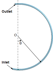
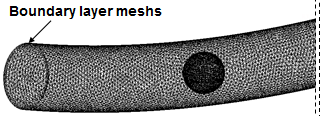
One identical mesh model is used in both the steady and the transient simulations. The meshes near the ball surface and the tubing wall are as dense as possible when the flow zone is discretized. Four boundary layers are arranged near the tubing internal wall, which expanded with an expansion coefficient of 1.2. The ball-tubing model is shown in Figure. 2. The central angle of the tubing is 210 ° in a counter-clockwise direction beginning from the vertical downward line. The initial ball center and the tubing inlet lie at 0 º and -20 °respectively, which ensures that the incoming flow can fully develop. Other parameters include: coiled tubing with an inner diameter of 63.425 mm, curvature radius of tubing center line of 1.268 m, a solid ball diameter of 40 mm, and a ball density of 7800 kg/m3.
Furthermore, the simulation was required to be independent with the element number of a mesh model, so the steady simulation was performed with different sizes of mesh. The research results demonstrated that the tangential fluid force exerted on the ball changed slightly once the total number of the element was as high as 1.2 million, and the qualified mesh model was adopted in the following simulation:
Figure 2. Ball structure and grid model
The SIMPLE and PISO algorithms [12] were used in the steady and transient simulations respectively, and the force on the ball was calculated to determine the ball’s transient velocity and displacement based on the flow simulation. The mesh was updated at the end of each step with dynamic grid technology in the transient simulation, and the new mesh was adopted for simulation at step. The above steps were repeated until the ball arrived at the tubing outlet.
Considering that a zero or negative volume may exist if the displacement of the ball within a single time step is larger, the time step Δt was determined to guarantee calculation convergence based on the ball’s moving speed and the grid size, and 0.001 s was set. The boundary conditions included: velocity inlet at the tubing inlet, pressure outlet at the tubing outlet, and no slip wall boundaries.
4.1 Steady flow field and fluid force
Fresh water was pumped into the tubing with a density of 1000 kg/m3 and viscosity of 0.001 Pa×s. Assuming that the ball center coincided with the tubing center, the flow field at the gravity is shown in Figure. 3.
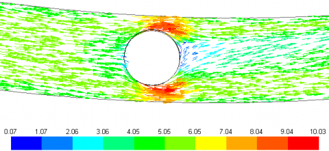
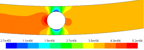
Figure. 3a shows that the fluid skirted the static ball and reached the maximal velocity value of 9800 Pa at the gap between the ball and tubing inner wall. Obviously, the phenomenon of flow boundary layer separation happened at the ball’s rear, causing an increase in the rear pressure (as shown in Figure. 3b).
a Flow velocity (m/s)
b Fluid pressure (Pa)
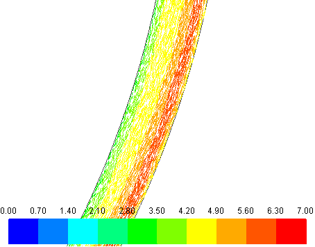
Figure 3. Flow field around the ball (inlet velocity 5 m/s, θ= 0°)
a Flow velocity (m/s)
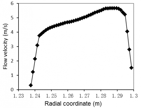
b Flow velocity on the cross section
Figure 4. Flow field away from the ball (inlet velocity 5 m/s, θ= 0 °)
Figure. 4a shows that the flow velocity vector away from the ball changed significantly along the radial direction, indicating the far field is hardly affected by the ball. Due to the centrifugal force, the velocity increased from the inner wall of the tubing to the outer wall, and decreased sharply near the tubing outer wall because of the wall effect (as shown in Figure. 4b).
As a result of the uneven flow, a radial lift force was created to force the ball to move outward.
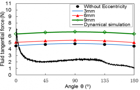
Figure. 5 shows the liquid tangential force when the ball was outwardly eccentric relative to the tubing center. The force acted on the ball changed inconspicuously with different θ, and reached the maximum when θ was 90 °. On the other hand, the tangential force increased with the increase of eccentricity. As the tangential force was larger than the tangential component of the gravity, it can be presumed that the ball has the tendency to move ahead. Additionally, the fluid forces computed from the transient simulation were much smaller compared with the steady simulation; the minimum occurred at 180 °, which indicates that judgment of whether or not the ball passes through the coiled tubing cannot be attained with steady simulation.
Figure 5. Tangential fluid force exerted on the ball
4.2 The transient flow field and the ball motion rule
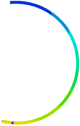
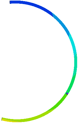
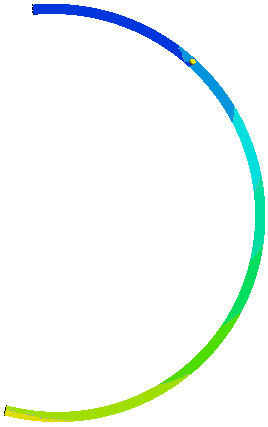
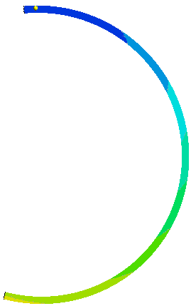
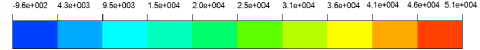
Figure 6 shows the ball movement and pressure field after the ball entered from the tubing inlet. The ball moved along the outside surface inner tubing to arrive at the highest point, indicating that the ball can pass through the tubing-wound coiling block when the flow velocity is 5 m/s. The movement of the ball had little influence on the far field, and the pressure continuously decreased with the increase of θ under the effect of gravity.
0.50s
0.01s
1.0s
1.25s
Figure 6. Ball instantaneous position and pressure field (Pa)
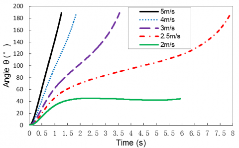
The angular displacement and angular velocity of the ball under different flow velocities are shown in Figures. 7 - 8. Figure. 7 shows that the ball could quickly reach the point at 180 ° as the flow velocity was greater than 3 m/s, and the ball retained a static balance at about 42 ° because of the zero velocity of the ball when the flow velocity was reduced to 2 m/s (as shown in Figure. 8).
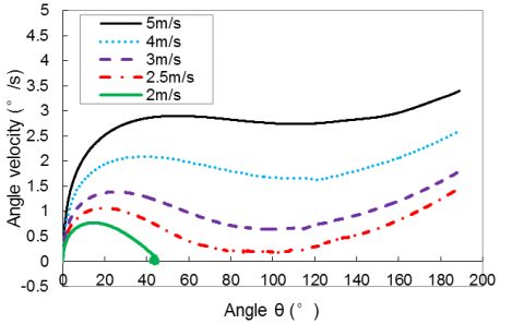
The condition for the ball to rotate around the tubing curvature center is to overcome the tangential component of gravity. Figure. 8 shows that with an increase of θ, the ball started to move quickly, and then decelerated to the minimum of about 90 ° because the tangential component of gravity Fg·sinθ was gradually enhanced. Subsequently, the angular velocity increased for a reduction of Fg·sinθ when θ > 90 °. When θ > 180 °, the angle velocity increased further because gravity turned to speed up the ball, and the ball moved faster at the corresponding angle of the tubing inlet, indicating that the ball would reach the highest position and eventually pass through the whole tubing once it had passed through the location of 90 ° in the first winding. So, we regard the minimum velocity, which happened at 90 °, as the critical velocity at which the ball can pass through the coiled tubing.
Figure 7. Angular displacement of ball revolving round the tubing curvature center
Figure 8. Angular velocity of ball revolving round the tubing curvature center
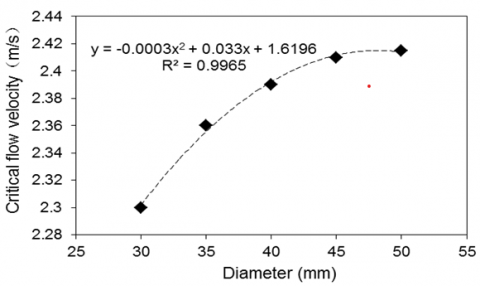
Figure 9. Critical flow velocities for the different size balls
The critical flow velocities for different size solid balls are shown in Figure. 9. It demonstrates that the critical velocity increased from 2.3 m/s to 2.415 m/s when the ball diameter increased from 30 mm to 50 mm, which approximately obeyed a quadratic polynomial.
In summary, we have simulated the flow of coiled tubing wrapped around a coiling block, using CFD with steady and transient methods. Basing on the flow simulation, the fluid force on the ball has been computed, and the ball movement has been determined.
(1) The fluid force on the static ball was related to θ for the gravity, and the maximal tangential component appeared at θ = 90°, which increased in line with the increase of ball-tubing eccentricity. For the centrifugal inertia, the maximum flow velocity far away from the ball appeared near the outer wall of the tubing.
(2) With the dynamic grid method and the simplification of impact, we have simulated the ball movement and the flow, and found that the fluid force acting on the moving ball was much smaller than that of the steady simulation, which was in conformity with the reality.
(3) The ball velocity around the curvature center of tubing increased from 0 and then decreased to the minimum at θ = 90°, but nevertheless rose again. This indicates that the ball can arrive at the highest position and even pass through the entire coiling block if the ball velocity is larger than zero at θ = 90° at the first winding. Additionally, as the diameter of the solid ball was increased from 30 mm to 50 mm, the critical flow velocity of the ball rose from 2.30 m/s to 2.415 m/s with the law of quadratic curve.
Through this study, the feasibility of CFD for simulating the ball passing through a section of coiling block of the tubing was verified, and a scientific basis for determinating the subsequent experimental parameters was provided.
This study was supported by the Natural Science Foundation of Hubei (2015CFC858) and the Doctoral Fund of E Education Ministry (20114220110001).
1. R.D. JONES, Developing Coiled-tubing Techniques on the Karachaganak Field, Kazakhstan, SPE 68349, 2001. DOI: 10.2118/0601-0030-JPT.
2. S.B. Lonnes, K.J. Nygaard, W. A and R. Tolman Sorem, Advanced Multi-Zone Stimulation Technology, SPE 95778, 2005. DOI: 10.2118/95778-MS.
3. X. Li, Z. Chen, S and Chandhary, An Integrated Transport Model for Ball-sealer Diversion in Vertical and Horizontal Wells, SPE 96339, 2005. DOI: 10.2118/96339-MS.
4. Ramadan, P. Skalle, A. Saasen, “Application of a three-layer modeling approach for solids transport in horizontal and inclined channels,” Chemical Engineering Science, vol. 60, pp. 2557-2570, 2005. DOI: 10.1016/j.ces.2004.12.011.
5. H. Xiao, J. Li, J. Zeng, “Ball Motion Equation in the Ball Sealer Fracturing,” Journal of Southwest Petroleum University (Science & Technology Edition), vol. 33, pp. 162-167, 2011. DOI: 10. 3863/j. issn.
6. Z.H. Shen, H.Z. Wang, G.S., “Numerical simulation of the cutting-carrying ability of supercritical carbon dioxide drilling at horizontal section,” Petroleum Exploration and Development, vol. 38, pp. 233-236, 2011. DOI: 10.1016/S1876-3804(11)60028-1.
7. S.P. Engel, P. Rae, New Methods for Sand Cleanout in Deviated Wellbores Using Small Coiled Tubing, SPE 77204, 2002. DOI: 10.2118/77204-MS.
8. V.C. Kelessidis, G.E. Bandelis, Flow Patterns and Minimum Suspension Velocity for Efficient Cuttings Transport in Horizontal and Deviated Wells in Coiled-tubing Drilling, SPE 81746, 2004. DOI: 10.2118/81746-MS.
9. R. Rooki, F. Doulati Ardejani, A. Moradzadeh, V.C. Kelessidis and M. Nourozi, “Prediction of terminal velocity of solid spheres falling through newtonian and non-newtonian pseudoplastic power law fluid using artificial neural network,” International Journal of Mineral Processing, vol. 110-111, pp. 53-61, 2012. DOI: 10.1016/j.minpro.2012.03.012.
10. A.B. Basset, Hydrodynamics, chap. 2, Dover Press, New York, 1961.
11. Bonfiglioli and R. Paciorri, “A local, un-structured, re-meshing technique capable of handling large body-motion in rotating machinery,” Energy Procedia, vol. 82, pp. 209-214, 2015. DOI: 10.1016/j.egypro.2015.12.022.
12. Z. Hu, W.Y. Tang, H.X. Xue, X.Y. Zhang, “A SIMPLE-based monolithic implicit method for strong-coupled fluid–structure interaction problems with free surfaces,” Computer Methods in Applied Mechanics and Engineering, vol. 299, pp. 90-115, DOI: 10.1016/j.cma.2015.09.011.