OPEN ACCESS
The aim of this work is the analysis, under dynamic conditions, of the energy performance of buildings based on different climatic conditions. Two school buildings, Liceo Classico “E. Duni” and Liceo Scientifico “D. Alighieri”, located in Matera, Italy, are considered. Furthermore, a strategy to improve the energy performance of the two school buildings is proposed by the installation of a co-trigeneration plant integrated with a solar plant. Such a plant is equipped with an absorption chiller to produce chilled fluid. The analysis under dynamic conditions has been performed by using a well-known simulation software, TRNSYS 17, and the results have been compared with those obtained under stationary conditions by employing a numerical solver, MC-11300, which is certified by the Italian Thermotechnical Committee. At first, the results obtained by considering the dynamic and stationary states and the experimental data measured in situ are compared by considering the actual buildings plants. Then, the energy performance of the two buildings is computed by considering three different climatic zones of Italy. Finally, a discussion of the advantages of the proposed requalification solution, which employs the trigeneration plant, is given. (Presented at the AIGE Conference 2015)
Dynamic simulation, Energy performance, School building, TRNSYS model, Trigeneration.
Recently, the exploitation of local energy sources and the adoption of local energy generation systems are fundamental issues dealing with energy conversion systems. On the other hand, the employment of cogeneration systems enables the simultaneous production of electricity and heat from a single source. Cogeneration plants are composed of combined heat and power systems with an electric output [1, 2]; this type of plant is known for its good overall efficiency in terms of resources consumption with respect to the separate production of the same cogenerated energy vectors [3, 4]. Co-trigeneration plants [5] represent the further evolution of cogeneration plants [6] with a global improvement of the plant performance. They satisfy heating, cooling and electrical requirements from the same source of energy [7], by using some of the produced heat to generate chilled fluid with an absorption chiller. To enhance the plant performance, co-trigeneration plants integrated with a solar plant are currently under investigation [8-10].
The aim of this work is the analysis of the energy performance of two school buildings, in order to optimize their performance and efficiency. The whole system is simulated by TRNSYS 17 simulation software [11-14]. Such a software has several advantages, i.e. a good technical documentation, the availability of the source code, the modular design, which allows representing buildings and plants through components (types), and, finally, the ability to link to other codes. On the other hand, the weaknesses are represented by a resolution technique of the thermal exchanges based on the “z–transfer function”, which makes the modeling of building envelopes with high thermal inertia a difficult task, and a simplified model through the “star temperatures” of the inner surfaces of the thermal zones [15]. By comparing the results obtained with TRNSYS and Energy Plus Software (EPS) [16] under dynamic conditions, it is shown that EPS results in the highest net heating demand, while TRNSYS calculates the lowest. However, the difference between the two softwares in terms of outputs is less than 4%.
Two school buildings [17], Liceo Classico “E. Duni” and Liceo Scientifico “D. Alighieri”, in Matera, Italy, are analysed. The results obtained under dynamic conditions [18] are compared with those under stationary conditions obtained by employing MC-11300, which is a numerical solver certified by the Italian Thermotechnical Committee. Under stationary conditions, the simulations of the energy performance of the buildings do not provide an accurate prediction of the real energy performance, since such simulations do not consider the periodic variation of temperature and of solar radiation, but employ daily averaged weather data. On the other hand, under dynamic conditions [19], more careful and detailed studies can be performed to assess building envelope performances with different external factors, such as outside temperature, solar radiation, natural ventilation, users’ behavior and air conditioning plant. Moreover, according to the current Italian legislation (Legislative Decree 311/2006 and the application of new regulations – DM 06/26/2015) and the new UNI TS 11300 regulations “Energy performance of buildings” Part 1-2-3-4, studies from now on will be based on hourly weather data rather than monthly averaged weather data, thus obtaining more accurate results and highlighting specific conditions.
In this work, several analyses under dynamic conditions are carried out by changing the number of days when the heating plant is working. Specifically, the number of heating days is reduced by considering the real operating conditions of the two schools [20]. The results of the simulations, in terms of energy performance, under stationary and dynamic conditions are compared [1, 2, 16]. Furthermore, the simulation results are compared with the experimental data in terms of thermal energy demand measured in situ, thus validating the model. Then, the model is used to predict the energy performance of the two buildings under climate conditions different from those of Matera. Specifically, three different cities of Italy, i.e. Bolzano, Rome and Palermo, are considered to account for typical climatic conditions of northern, central and southern Italy.
Finally, a strategy to improve the energy performance of the two buildings is proposed. Such a strategy consists of the installation of a co-trigeneration plant integrated with a solar plant. Specifically, the co-trigeneration plant is composed by two internal combustion gas engines connected in parallel so that the sum of their power satisfies the maximum requirement for heating and electrical power. This plant is equipped with an absorption chiller to produce chilled fluid. The reason for the choice of this design is based on the potential efficiency of using part of the cogenerated thermal power to heat the absorption machine for cooling production, enabling better exploitation of the global system plant.
This work is organized as follows: first the main features of the two buildings are given, then the simulation model is described and the results are discussed. A requalification solution with a trigeneration plant is given and finally the conclusions are summarized.
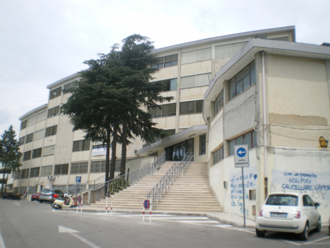
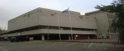
This study deals with the energy performance of two school buildings, Liceo Classico “E. Duni” and Liceo Scientifico “D. Alighieri”, in Matera, Italy, built of reinforced concrete in the mid 60s and early 70s, respectively.
Liceo Classico “E. Duni” is made up of five levels above the ground level and one basement level, with a total volume of 21,800 m3 and a surface area of 6,085 m2. The current heating system is fueled with natural gas boiler; the natural gas consumption amounts to 57,680 m3/year. The electricity consumption is equal to 79,242 kWh/year. The lighting plant is made up of 439 neon distributed in several rooms of the school building. Currently, Liceo Classico “E. Duni” has a unique heating system located in a central position of the building (to balance the distribution network). There is a boiler room with two heat generators built in 2006. The heat generator consists of two basic components: the burner and the boiler itself. The burner supplies the required fuel quantity into the boiler combustion chamber where the combustion between fuel and oxygen takes place. The heat transfer fluid is water and radiators emission system is used. The thermal power is equal to 340 kW with an efficiency of 92% (operating at full load). The actual energy consumption of Liceo “E. Duni” has been monitored in the four-year range 2009-2012.
Liceo Scientifico “D. Alighieri” is made up of four levels above the ground level, with a total volume of 44,851 m3 and a surface area of 7,830 m2. The current heating system is fueled with natural gas boiler; the natural gas consumption amounts to 23,546 m3/year. The electricity consumption is equal to 39,532 kWh/year. The lighting plant is made up of 366 neon distributed in several rooms of the school building. Liceo Scientifico “D. Alighieri” has a unique heating system located next to the building. The heat transfer fluid is water and a radiators emission system is employed. The heating system is composed of five thermal generators (Type 1), installed about a year ago with a total power of 908 kW and one thermal generator (Type 2), installed about a year ago with a total power of 147 kW.
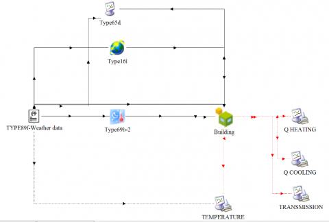
The dynamic model used to simulate the whole system has been developed by employing TRNSYS 17 software. The layout is shown in Figure 1. The model is composed of the following parts: weather data reader and radiation processor, psychrometric processor, solar radiation processor and building model. The weather data reader takes data from input file in .EPW format and processes the global radiation to compute several quantities related to the position of the sun, and to estimate insolation on a number of surfaces of either fixed or variable orientation. The psychrometric processor takes as input the dry bulb temperature and relative humidity of moist air and returns the corresponding moist air properties, i.e. dry bulb temperature, dew point temperature, wet bulb temperature, relative humidity, absolute humidity ratio, and enthalpy. Moreover, it determines an effective sky temperature, which is used to calculate the long-wave radiation exchange between an arbitrary external surface and the atmosphere. The effective sky temperature is always lower than the current ambient temperature. The black sky on a clear night, for example, is assigned a low effective sky temperature to account for the additional radiative losses from a surface exposed to the sky. The solar insolation data is generally taken at one hour intervals and on a horizontal surface. The solar radiation processor interpolates radiation data, calculates several quantities related to the position of the sun, and estimates insolation on a number of surfaces of either fixed or variable orientation. The building model simulates the thermal behaviour of a building composed of different thermal zones. The processor generates its own set of monthly and hourly summary output files.
The whole system has been simulated by using a simulation time step equal to 1-hour, with a duration of the simulation period depending on the city under consideration.
3.1Model set-up for Liceo Classico “E. Duni”
The entire building is divided in two types of thermal zones, so that different indoor comfort conditions may be set, depending on the use of the rooms, i.e. restrooms as bathrooms, hallway and stairway and classrooms that include every room intended for the development of school activity, by considering also laboratories and meeting rooms. The two thermal zones are defined for each floor. Therefore, by considering that the school building is made up of 6 levels, 12 different thermal zones are obtained.
Even though the model allows to manage the two thermal zones independently of one another, in this work the actual plant is simulated, so the same conditions for the two thermal zones are imposed. Specifically, the internal temperature (set-point temperature) is set to 20°C, whereas the heating demand profile is shown in Figure 2.
The building envelope, shown in Figure 3, is made up of the external wall, which is the larger component of the building envelope and is made of concrete blocks plastered on both sides, the windows, which are of three types:
Figure 1. Simulation model with TRNSYS 17
Figure 2. Heating demand profile – operating plant
Figure 3. Building envelope of Liceo Classico E. Duni
Figure 4. Building envelope of Liceo Scientifico D. Alighieri
►North, east and west façade, south façade of first floor: made of metal frames without thermal insulation (thickness of 3 cm) with single glass and characterized by a high transmittance value; most of them are devoid of shutters;
►South façade of basement floor, some elements of north façade of basement floor: made of metal frames without thermal insulation (thickness of 5 cm) with single glass and characterized by an average transmittance value; most of them are devoid of shutters;
►Some elements of south and north façade of basement floor: made of metal frames without thermal insulation (thickness of 5 cm) with double glass (4-6-4 mm) and characterized by a low transmittance value; most of them are devoid of shutters;
the basement horizontal floor, which is in contact with the ground and the roof floor, which is not accessible. Since there are not enough data for an accurate definition of the floors, the Italian Heat Technology Committee schedule [21] is used as reference, assuming the floor against the earth is made of lightweight concrete and stoneware interior flooring and the roof floor is made of concrete base and brick blocks.
3.2Model set-up for Liceo Scientifico “D. Alighieri”
The building envelope, shown in Figure 4, is made up of the external wall, which is the larger component of the building envelope and is made of concrete blocks plastered on both sides, the windows, which are made of metal frames without thermal insulation with single glass, are characterized by a high transmittance value and most of them are devoid of shutters, the basement horizontal floor, which is in contact with the ground, the floor against the earth, made of lightweight concrete and stoneware interior flooring, and the roof floor, which, according to the Italian Heat Technology Committee schedule [21], is assumed to be made of concrete base and brick blocks.
Also in this case, two thermal zones are enabled for each level, but in this work the same conditions for the two zones are imposed.
4.1 Model validation
In order to validate the model set-up, simulations of the energy performance of Liceo Classico “E. Duni” have been carried out by considering the weather conditions of the city of Matera. The Italian regulations divide the country in different climatic zones according to the average meteorological conditions for each town. Therefore, different climatic zones indicate different weather conditions. Specifically, the calculations have been carried out by considering the hypotheses given in Table 1 for the city of Matera.
Table 1. Climatic conditions and hypothesis for the model validation
|
City |
Climatic zone |
Heating period |
Operation of the plant |
|
Matera |
D |
1st November ÷15th April |
12 hour/day |
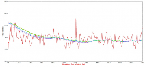
Figure 5. Internal and external temperatures – behavior without heating plant (January)
The results of the simulations performed under dynamic conditions are compared in Table 2 with those obtained under stationary conditions by employing MC-11300 software [22] and with the actual data measured in-situ. Specifically, TED and EPI indicate the Thermal Energy Demand for heating and the Energy Performance Index, respectively.
The results obtained under dynamic conditions show a deviation of about 32% compared to the data obtained under stationary conditions and are closer to the actual data with respect to stationary conditions results, thus showing the importance of considering the time variation of the different parameters (first of all the thermal inertia and the envelope storage capacity). The calculation under stationary conditions is not only misleading with respect to the actual operating conditions of the buildings but also is not reliable in energy requalification proposal. This is the reason why the latest updates of the Italian legislation on energy performance of buildings – D.M. June 26, 2015 – provide that the calculation of the energy performance has to be carried out on hourly data and not on a monthly average. The dynamic conditions results are, however, considerably different with respect to the actual consumption with a deviation of 86%. Such a difference may be due to the choice of the operating conditions, since, in agreement with law disposal, it has been supposed that the heating plant works 12 hr/day, whereas 8 hr/day seems to be a more reliable hypothesis. The computations have been repeated under this new assumption and the results are given in Table 3. In this case the result shows a deviation of about 61%. This value is rather high yet. A further simulation has been carried out by considering that the school is closed during holidays. So the heating period decreases from 166 days to 121 days. In this case the thermal energy demand for heating under dynamic conditions is similar to the actual consumption: indeed the deviation between the two results reduces to about 17%, as shown in Table 4. Such a difference is considered acceptable within the present work to validate the model.
Figure 5 shows the outside temperature (red line) and the internal temperatures of the different thermal zones (remaining lines) in January, when the heating plant is turned off. The diagram shows that the internal temperatures of the heating zones follow the trend of the external temperature with a time delay which depends on the thermal inertia of the building envelope. In the specific case, it is noted that the school building is characterized by a sufficient thermal inertia when the operating condition is reached: the variation of the internal temperature is about 3,5 °C while the value of the average temperature is about 5,4 °C.
Table 2. Results referred to the city of Matera (model validation – Liceo Duni) - heating period 1st November÷15th April – 12 hr/day
|
|
Stationary conditions |
Actual data |
Dynamic conditions |
|
TED [kWh] |
555,492.52 |
226,041.60 |
420,871 |
|
Heated useful floor area [m2] |
4,814.06 |
4,814.06 |
4,814.06 |
|
Gross heated volume [m3] |
15,467.43 |
15,467.43 |
15,467.43 |
|
EPI [kWh/ m3 year] |
35.914 |
14.65 |
27.21 |
Table 3. Results referred to the city of Matera (model validation – Liceo Duni) - heating period 1st November÷15th April – 8 hr/day
|
|
Actual data |
Dynamic conditions |
Deviation |
|
TED [kWh] |
226,041.60 |
363,202.45 |
60.68% |
|
EPI [kWh/ m3 year] |
14.61 |
23.48 |
Table 4. Results referred to the city of Matera (model validation – Liceo Duni) - heating period 1st November÷15th April and 121 day– 8 hr/day
|
|
Actual data |
Dynamic conditions |
Deviation |
|
TED [kWh] |
226,041.60 |
264,743.96 |
17.12% |
|
EPI [kWh/ m3 year] |
14.61 |
17.11 |
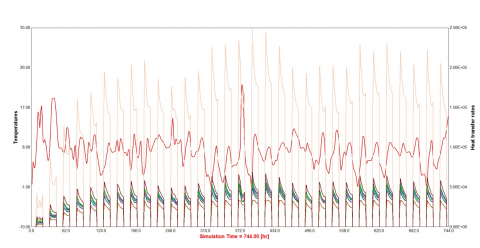
Figure 6 shows the outside temperature (red line indicated by the arrow) and the hourly averaged power for the different thermal zones (remaining lines) in January when the heating plant is on. Specifically, the pink line refers to a zone on the upper floor with high dissipation loss. As expected, the trend of energy consumption is similar to the heating demand profile shown in Figure 2 (during the 24 hours of each day). Moreover, the energy consumption varies with the external temperature conditions, being higher when the outside temperature is lower. Figure 6 allows to evaluate the quality of building envelope thermal inertia. Indeed, as soon as the plant switches on, there is a higher power consumption because the heating system should guarantee the achievement of the set point temperature starting from an internal temperature rather low (overnight internal temperature). During the 12 hours of plant operations, consumptions tend to decrease: the heating system, in fact, has to maintain the indoor temperature set point that is reached in the first hours when the plant is switched on. Although the heat loss increases with the difference between internal and external temperatures, the envelope delays the heat transfer as much as it is equipped with thermal inertia.
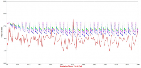
Figure 7 shows the trend of the internal and external (red line) temperatures when the heating system is on. From the figure, the set-up of plant operations (12 hours a day – Tset, point = 20°C) is evident. When the heating system turns off, the slope of the curves indicates the ability to maintain over time the heat accumulated during the heating system operations.
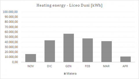
Figure 8 shows the monthly energy consumption in the period 1st November ÷15th April considered for the simulation. As expected the energy consumption varies with the external temperature conditions, being higher in January when the outside temperature is low. April is characterized by low heating consumption as the heating system is turned on for only 15 days and outside temperatures are milder. November has reduced energy requirements even if the outside temperatures are rather low, since the building envelope is still “hot” after the summer months.
Figure 6. Energy consumption – behavior with heating plant (January)
Figure 7. Internal and external temperatures – behavior with heating plant (January)
Figure 8. TED per month for Liceo Duni under dynamic conditions
4.2 Influence of climatic conditions on different buildings
In order to analyze the behavior of the school buildings under different climatic conditions, three Italian cities, i.e. Bolzano, Rome and Palermo, characterized by climatic conditions quite different from each other, have been considered. The energy performance of the two school buildings has been computed under the assumption they were located in the three cities. Specifically, the calculation under stationary conditions and dynamic conditions has been carried out by considering the hypotheses given in Table 5 and the results are shown in Table 6.
As expected, the results for both schools show that the energy consumption decreases by performing the simulation in the center and, even more, in the south of Italy with respect to the same computation carried out in northern Italy. Besides, under stationary conditions a higher TED and EPI for Liceo D. Alighieri with respect to the other school is obtained. The EPI of Liceo D. Alighieri is about 2.04/1.41 times the EPI of Liceo Classico E. Duni by considering the city of Palermo/Bolzano. Under dynamic conditions the EPI of the two buildings is comparable for all the three cities.
By comparing the stationary and the dynamic results in terms of TED it is shown that under stationary conditions the results are always overestimated, with the higher differences occurring in the case of Liceo Alighieri. In this case, the differences between stationary and dynamic conditions are higher in warmer weather conditions (Palermo) compared to colder climates and temperature (Bolzano). This result is probably due to the effects of the building envelope and thermal inertia, which are more accurately computed in the dynamic simulation.
Moreover, an assessment of the actual energy consumption of the two school buildings, as if they were located in the other three Italian cities, can be performed. Table 7 shows the results, for Liceo Duni and Alighieri of the dynamic simulations performed in the three cities under the hypothesis used in the model validation, i.e. by considering that the school is closed during holidays, thus reducing the heating period of 45 days in a year with respect to the set-up given in Table 5. Then, the actual consumption has been assessed by assuming that the deviation between the data obtained from the dynamic simulation and the hypothetical actual consumption is constant in the three locations and equal to about 17%. The results, named consumption assessment, are shown in Table 7.
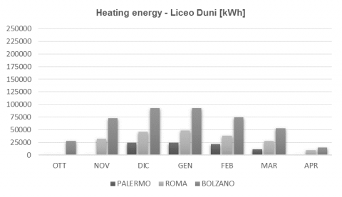
Figure 9 shows the monthly TED for both buildings in the three different locations computed by using the dynamic simulation under the hypotheses given in Table 5. The results are consistent with the specific climate conditions of the three cities, with the higher energy consumption on December and January.
Table 5. Climatic conditions and operation hypotheses
|
City |
Climatic zone |
Heating period |
Operation of the plant |
|
Bolzano |
E |
15th October ÷ 15th April |
14 hour/day |
|
Rome |
D |
1st November ÷ 15th April |
12 hour/day |
|
Palermo |
B |
1st December ÷ 15th March |
8 hour/day |
Table 6. Results referred to the cities of Bolzano, Rome and Palermo (stationary and dynamic conditions)
|
|
Liceo E. Duni |
Liceo D. Alighieri |
||
|
|
TED [kWh] |
EPI [kWh/ m3 year] |
TED [kWh] |
EPI [kWh/ m3 year] |
|
|
stationary conditions |
|||
|
Bolzano |
911,052.70 |
58.90 |
3,713,689.14 |
82.8 |
|
Rome |
424,244.34 |
27.43 |
2,055,712.40 |
45.8 |
|
Palermo |
196,925.84 |
12.73 |
1,170,862.28 |
26.1 |
|
|
dynamic conditions |
|||
|
Bolzano |
691,031.31 |
44.68 |
2,175,150.83 |
48.48 |
|
Rome |
326,635.13 |
21.12 |
861,740.87 |
19.21 |
|
Palermo |
130,991.29 |
8.47 |
376,781.30 |
8.40 |
Table 7. Results referred to the cities of Bolzano, Rome and Palermo - 8 hr/day – Energy consumption assessment
|
TED [kWh] |
Heating period |
Dynamic conditions |
Consumption assessment |
|
|
|
|
Liceo Duni |
||
|
Bolzano |
15st October÷15th April [137 days] |
405,154.03 |
345,930.70 |
|
|
Rome |
1st November÷15th April [121 days] |
202,177.10 |
172,623.89 |
|
|
Palermo |
1st December÷31th March [76 days] |
84,861.69 |
72,457.05 |
|
|
|
|
Liceo Alighieri |
||
|
Bolzano |
15st October÷15th April [137 days] |
1,247,660.27 |
1,065,283.70 |
|
|
Rome |
1st November÷15th April [121 days] |
590,672.53 |
504,331.05 |
|
|
Palermo |
1st December÷31th March [76 days] |
247,828.57 |
211,602.26 |
|
Figure 9. TED per month under dynamic conditions
In details, the trigeneration plant is composed of: a cooling tower, which is a heat exchange device that allows the transfer of heat substantially without increasing the air temperature but exploiting the heat of evaporation of water yielding only steam into the atmosphere; an absorbtion liquid chiller, which uses waste heat of the cooling tower in order to
refrigerate heat transfer fluid; an internal combustion engine, which consists of two engines, with power equal to 365 kW and 210 kW, respectively, connected in parallel so that the sum of their power satisfies the maximum need of heating thermal power and electrical power of the two schools; solar thermal collectors; heat exchangers; storage tanks; hydronics.
Figure 10. Trigeneration plant layout
The efficiency and the energy saving of the trigeneration plant can be estimated on the basis of the scientific literature [2, 3, 23-25]. Specifically, in [2], the authors examine the performance of a residential building-integrated micro-cogeneration system during the winter by using TRNSYS. The influence of the most significant boundary conditions on the system environmental and economic performance were analyzed by running simulations with different volumes of the hot water storage, different climatic zones, different electric demand profiles, and different type of micro-cogeneration unit control strategies (electric load-following and thermal load-following operation). The analyses showed that whatever the city and the control logic are, the hot water tank with the largest volume allows for minimizing the equivalent carbon dioxide emissions, as well as the operating costs of the system. Whatever the city and electric demand profile are, the proposed system allows for a reduction of equivalent carbon dioxide emissions in comparison to the reference system only in the case of thermal load-following logic; the alternative system is more convenient than the conventional system from an economic point of view whatever the city, electric demand profile and MCHP control logic are.
Based on this analysis, it appears that the adoption of a cogeneration system would be useful also in the case studied in this work, to reduce the emissions of carbon dioxide. In particular, it emerges that an important factor for the evaluation of system efficiency is the size of the storage tank and the energy system management and control. Moreover, the system turns out to be economically viable for any case, even if the best results are obtained in colder climatic conditions.
In the present work, the summer mode is also very interesting by considering that the school buildings could be used for other activities and that Matera is characterized by rather warm summers. Besides, to ensure suitable indoor comfort, it is essential to promote strategies that allow thermohygrometric control within school buildings. For this reason, a trigeneration plant is proposed in this work.
This paper deals with the investigation of the energy performance of two school buildings in the city of Matera, Italy, under stationary and dynamic conditions. At first, the model has been validated by comparing the computations, in terms of energy consumption, with the actual data measured in situ. By assuming that the plant works in the period 1st November ÷15th April for 12 hours/day, both stationary and dynamic simulations overestimate the actual energy consumption, with the stationary consumption higher with respect to the dynamic consumption, with a difference of about 32%, that is in agreement with the scientific literature. By assuming that the plant is turned on in the period 1st November÷15th April for only 121 days for 8 hrs/day, the dynamic simulations are in good agreement with the actual data, with a difference of about 17%. Such a difference is deemed acceptable, by considering that the available experimental data is a global parameter, i.e. the energy consumption over the whole year, and that the effective operating conditions of the plant are not known in details. Then, the computational model has been used to predict the energy performance of the two schools under different weather conditions in three different climatic zones of Italy. As expected, the results for both schools show that the energy consumption decreases by performing the simulation in the center and, even more, in the south of Italy with respect to the same computation carried out in the northern part of Italy. Besides, the energy performance index is different for the two schools examined in this work, since the thermal inertia of the buildings envelope is different. Finally, a strategy is proposed to improve the energy performance of the two school buildings. A trigeneration plant, that allows the simultaneous production of heat, cool and power energy, is designed and shown in the paper.
Financial support has been received through the Project FESTA (Fostering local energy investments in the Province of Matera). Furthermore, this project has received funding from the European Union’s Horizon 2020 Research and Innovation Programme under Grant Agreement No 649956.
1. A. Rosato, S. Sibilio, M. Scorpio, “Dynamic performance assessment of a residential building-integrated cogeneration system under different boundary conditions. Part I: Energy analysis,” Energy Conversion and Management, 79, pp. 731–748, 2014. http://dx.doi.org/10.1016/j.enconman.2013.10.001.
2. A. Rosato, S. Sibilio, M. Scorpio, “Dynamic performance assessment of a residential building-integrated cogeneration system under different boundary conditions. Part II: Environmental and economic analyses,” Energy Conversion and Management, 79, pp. 749–770, 2014. http://dx.doi.org/10.1016/j.enconman.2013.09.058
3. G. Chicco, P. Mancarella, “Trigeneration primary energy saving evaluation for energy planning and policy development,” Energy Policy, 35, pp. 6132–6144, 2007. http://dx.doi.org/10.1016/j.enpol.2007.07.016
4. H.-M. Henning, T. Pagano, S. Mola, E. Wiemken, “Micro- trigeneration system for indoor air conditioning in the Mediterranean climate,” Applied Thermal Engineering, 27, pp. 2188–2194, 2007. http://dx.doi.org/10.1016/j.applthermaleng.2005.07.031
5. D. Sonar, S.L. Soni, D. Sharma, “Micro-trigeneration for energy sustainability: Technologies, tools and trends,” Applied Thermal Engineering, 71, pp. 790–796, 2014. doi:10.1016/j.applthermaleng.2013.11.037
6. M. Jradi, S. Riffat, “Tri-generation systems: Energy policies, prime movers, cooling technologies, configurations and operation strategies,” Renewable and Sustainable Energy Reviews, 32, pp. 396–415, 2014. http://dx.doi.org/10.1016/j.rser.2014.01.039
7. J. Wang, J. Wu, C. Zheng, “Analysis of tri-generation system in combined cooling and heating mode,” Energy and Buildings, 72, pp. 353–360, 2014. http://dx.doi.org/10.1016/j.enbuild.2013.12.053
8. M.U. Siddiqui, S.A.M. Said, “A review of solar powered absorption systems,” Renewable and Sustainable Energy Reviews, 42, pp. 93–115, 2015. http://dx.doi.org/10.1016/j.rser.2014.10.014
9. A. Rosato, S. Sibilio, G. Ciampi, “Dynamic performance assessment of a building-integrated cogeneration system for an Italian residential application,” Energy and Buildings, 64, pp. 343–358, 2013. http://dx.doi.org/10.1016/j.enbuild.2013.05.035
10. K. Gluesenkamp, Y. Hwang, R. Radermacher, “High efficiency micro trigeneration systems,” Applied Thermal Engineering, 50, pp. 1480-1486, 2013. doi:10.1016/j.applthermaleng.2011.11.062
11. Solar Energy Laboratory, TRNSYS 16, A Transient System Simulation Program, Tech rep. University of Wisconsin, Madison, USA, 2004.
12. D.B. Crawley, J.W. Hand, M. Kummert, B.T. Griffith, “Contrasting the capabilities of building energy performance simulation programs,” Building and Environment, 43, pp. 661–673, 2008. http://dx.doi.org/10.1016/j.buildenv.2006.10.027
13. M. Wetter, C. Haugstetter, “Modelica versus TRNSYS - A comparison between an equation-based and a procedural modeling language for building energy simulation,” Proc. of the 2nd SimBuild Conference, Cambridge, USA, Aug. 2006.
14. P. Caputo, M. Manfren, “Modelli per la simulazione energetica,” Report RSE/2009/59 ENEA, Roma, 2009.
15. C. Marinosci, G. Semprini, “Software di simulazione energetica dinamica degli edifici,” Sistema Integrato di Informazione per l’Ingegnere Inarcos n. 734/2013, 2013.
16. A. Buonomano, F. Calise, G. Ferruzzi, A. Palombo, “Dynamic energy performance analysis: Case study for energy efficiency retrofits of hospital buildings,” Energy, 78, pp. 555 – 572, 2014. http://dx.doi.org/10.1016/j.energy.2014.10.042
17. L. De Santoli, G. Caruso, F. Bonfà, I. Bertini, G. Puglisi, “Analisi dinamica del sistema edificio-impianto di un dipartimento universitario.,” Proceedings of the 64th Congresso nazionale ATI, L'Aquila, 2009.
18. M. Tonon, “Tecniche di simulazione dinamica per la determinazione del comportamento termico ed energetico degli edifici,” Ph.D. thesis, University of Padova, Padova 2004.
19. P. Baggio, F. Cappelletti, A. Gasparella, P. Romagnoni, “Il calcolo della prestazione energetica degli edifici: confronto tra i software per la certificazione,” Proceedings of the 63th Congresso nazionale ATI, Palermo, 2008.
20. J. Ortiga, J.C. Bruno, A. Coronas, “Selection of typical days for the characterization of energy demand in cogeneration and trigeneration optimization models for buildings,” Energy Conversion and Management, 52, pp. 1934–1942, 2011. doi:10.1016/j.enconman.2010.11.022.
21. UNI/TR 11552:2014, “Abaco delle strutture costituenti l’involucro opaco degli edifici – Parametri termofisici”.
22. A. Ninivaggi, “Riqualificazione energetica del polo liceale di Matera con impianti ad elevata efficienza,” Bachelor thesis, University of Basilicata, Matera, 2014.
23. J.H. Horlock, Cogeneration - Combined Heat and Power (CHP), 1997.
24. American Society of Heating, Refrigerating and Air-conditioning Engineers, ASHRAE HVAC Systems and Equipment Handbook, SI ed. ASHRAE, USA, 2000.
25. L.D. Danny Harvey, A Handbook on Low Energy Buildings and District Energy Systems, UK, 2006.