
Fatima H.A. AL-Janabi | Hussein A. M. Al-Zubaidi*
© 2026 The authors. This article is published by IIETA and is licensed under the CC BY 4.0 license (http://creativecommons.org/licenses/by/4.0/).
OPEN ACCESS
In water supply networks, free chlorine residuals in tap water are a major concern. This study applied Geographic Information System (GIS) and Inverse Distance Weighting (IDW) interpolation to explore the spatial distribution of free chlorine residuals in Al-Hilla District, Iraq. A total of 81 water samples from the distribution network were analyzed for pH, temperature, total dissolved solids (TDS), electrical conductivity (EC), turbidity, and free chlorine residual. The ranges were 7.3–8.9, 11.20–24.40 ℃, 563–732 mg/L, 1144–1489 µS/cm, 0.30–13.60, and 0.10–3.00 mg/L, respectively. Turbidity and free chlorine residual issues existed according to Iraqi, WHO, and EPA standards; however, pH, TDS, and EC met the standards. Free chlorine residual was inversely correlated with pH, with a Pearson coefficient of −0.26 and p < 0.05. Spatial mapping emphasized this correlation, showing low free chlorine residual concentrations at locations with high pH levels. Higher free chlorine residual concentrations, up to 3.0 mg/L, were located near the main pipes and water treatment plant (WTP), decreasing to 0.10 mg/L in other areas. These variations may be associated with distance from the plant, turbidity, chlorine dosage, leakages, illegal joints, and aging or damaged pipes. Infrastructure improvements and optimized chlorine dosage are recommended.
chlorine decay, chlorine residual, drinking water modeling, Geographic Information System, Inverse Distance Weighting interpolation, statistical analysis, tap water, water distribution system
The quality of tap water in residential areas is a main condition that guarantees the durability of human health. The persistent threats to global challenges restricting populations and resources have made water quality protection a requirement for sustainable development. Providing consumers with access to safe and clean water helps reduce mortality rates from pathogens. Thus, the management of water resources and their protection from pollution actually is a real investment in the future of humankind and the environment [1]. Chlorination is one of the most common and effective treatment methods used to prevent microbes and pathogens in tap water. Although free chlorine residual, the result of this process, is critical for water disinfection, an amount either above or below the internationally accepted threshold (0.2–5.0 mg/L) can have great health impacts on consumers [2, 3]. The chlorine concentration in drinking water decreases in the distribution network due to its total decay by reactions with organic matter and the inner surface of pipes. Therefore, the chlorination dosage takes into account this decrease in chlorine concentration, but the decay rate varies according to the concentration present in the water each time [4-7]. Hence, regulation of chlorine levels is the most important way to achieve water safety. In addition, monitoring and controlling its level within the permissible limits are necessary [8-10].
Monitoring of water quality and chlorine dosage is a significant strategy, so new research is focusing on developing sustainable, low-cost measurement techniques. This represents progress toward ensuring clean, healthy water delivery for the community [9]. Accordingly, many researchers have dealt with chlorine residual in tap water differently. For instance, Kulmedov et al. [11] analyzed chlorine residual decay across a water distribution system in Abuja, Nigeria, for risk-managed design and operation of water quality. Field data and statistical analysis were utilized to find the water quality parameters influencing chlorine decay in the distribution system. The results showed that the concentration of chlorine residual in the distribution system varied from 0.00 to 0.23 mg/L, which was generally lower than the EPA minimum permissible limit of 0.2 mg/L required for an effective water disinfection process. Spatial analysis of sampling sites, which ranged from 0 to up to 54 km from the treatment facility, also revealed notable differences in several water quality parameters. The statistical analysis results using correlation and principal component analysis (PCA) showed that the spatial distribution of chlorine residual concentrations decreases with distance from the disinfection station. Bahrudin et al. [12] analyzed chlorine residual concentration in drinking water distribution networks in Malang, Indonesia, and explored how distance and pH affect its spatial distribution. Data from 40 water samples collected from different points of the network were analyzed statistically using SPSS software and plotted spatially in ArcGIS software. Results showed that chlorine concentrations were highest near the reservoir (1.0 mg/L) and were lowest at the furthest points from the reservoir (0.1 mg/L). In addition, over 65% of network points fell below the permissible limits due to issues in the distribution pipes or long network distances. Correlation and regression analyses revealed a strong negative correlation between chlorine residual and distance. The pH value was also strongly negatively correlated with chlorine residual. Yousefi et al. [13] applied Geographic Information System (GIS) techniques in ArcView and statistical spatial analysis to explore and zone the chlorine residual spatial distribution based on samples collected from the water distribution system of Masiri City, Iran. The ANOVA analysis results showed that a statistically significant difference in residual chlorine level between the dry and wet seasons exists, and the levels were significantly lower during the dry season. Hence, microbiological contamination proved to be significantly higher during the dry season compared with the rainy season, which suggested a higher rate of pollution exposure under lower chlorine levels. It was found that chlorine residual becomes less than the permissible limits due to different reasons such as old pipes, low water pressure, and network length. Mohammadi et al. [14] used GIS to understand the spatial distribution effect of chlorine residual concentrations and pH on Trihalomethanes (THMs) formation at different locations in the distribution system. This distribution was zoned spatially using the Inverse Distance Weighting (IDW) interpolation. Hence, chlorine residual, pH, and THMs levels in the network ranged from 0.1–3.3 ppm, 8.1–8.6, and 40–59 ppb, respectively. It was noticed that a gradual decline happened in the chlorine concentration as distance from the treatment plant increased, and this may suggest an influence of pipe characteristics and water retention time on chlorine decay. Results also showed that the disinfection efficiency has a pH dependency, impacting the THMs formation. As pH becomes higher (usually greater than 8), hypochlorite ions (OCl⁻) increase and hypochlorous acid (HOCl) decreases. Furthermore, Arslan and Bagdatlı [15] performed spatial evaluation for several water quality parameters including chlorine residual in Ankara, Turkiye, for three years period (2018, 2019, and 2020). They employed spatial analysis using GIS and IDW to map the parameter concentration distribution. Based on the results, the chlorine residual ranged from 0.38 to 0.74 mg/L during the three years, obeying the permissible limits. This study's main finding highlighted the importance of statistical analyses using IDW and GIS in providing information for evaluating the chlorine residual as a water quality parameter in a water distribution network.
Unlike highly optimized or modern distribution networks, the free chlorine residuals in Al-Hilla District, Iraq, water distribution system haven’t been managed well due to lack of field data availability, intermittent supply schedules, fluctuating resources of water, old pipes, and rapid unplanned urban expansion. Although chlorine residual concentrations may fall below the permissible limits at any point in the water supply network for well-known reasons, continuously monitoring the network spatially helps control the disinfection process significantly, especially for regions where network pipes are not working efficiently or are old. Therefore, the objective of this work is to combine geospatial and statistical methods into a unified analysis to explore the spatial distribution pattern of free chlorine residual in tap water in a central region located in Al-Hilla District, Iraq, that hasn’t been previously evaluated using these methods. Moreover, the statistical relationship between free chlorine residual and some other water quality parameters will be highlighted in this region to show the significant parameters influencing the disinfection efficiency.
2.1 The study framework
Figure 1 displays a schematic representation of the study framework. The workflow steps start by selecting the study area to be explored and surveyed. In this study, the targeted study area was selected in which all neighborhoods are served by the same water treatment plant (WTP), ensuring that the free chlorine residual in all samples comes from a single source. The collected samples were transferred to the laboratory to be tested for the targeted water quality parameters, including pH, temperature, total dissolved solids (TDS), electrical conductivity (EC), turbidity, and free chlorine residual (chlorine). Hence, the dataset was prepared using MS Excel and then processed using R software for statistical analysis. Data exploration, correlation analysis, and trend detection were used to find the effect of water quality parameters on the chlorine spatial distribution. In addition, comparison with the water quality standard specifications was performed, showing the water supply network locations that failed to meet the standards. Finally, the dataset was imported into ArcGIS 10.8 for spatial analysis and IDW interpolation.
Figure 1. The study framework flowchart
2.2 The study area, sampling, and water quality measurements
The study was conducted at a central region (longitude: 44°25'30"E, latitude: 32°29'0"N, and area: 6.62 km²) situated in Al-Hilla District, the administrative center of Babylon Governorate, Iraq (Figure 2). The region is served by a water supply network receiving drinking water from a WTP called Al-Tayyara WTP. The plant is close to the Hilla River, the main water source in the district [16, 17]. Hence, raw water is drawn from the river, and then it is treated and pumped through the plant, providing treated potable water for this region of the district.
The network water quality was evaluated through an extensive field sampling campaign undertaken from March 3 to 24, 2026, consisting of the collection of 81 samples (N = 81) from the tap water at selected locations based on the network’s structure, geographic sector and neighborhoods, as shown in Figure 2. In addition, the sampling procedure included collecting an additional 28 samples from other locations used as a testing dataset for validating the IDW interpolation method. The sampling was mostly done during the daytime (between 08:00 and 16:00), covering residential houses, commercial premises, major roads and peripheral network branches. No repeat temporal sampling was conducted; only single samples were collected. There were some points in space that were geographically close to each other, but all relations were independent. Therefore, the maps obtained are a short-term spatial screening snapshot and not seasonal or annual variations. The water quality parameters were measured in situ at the sampling sites to maintain data collection accuracy for assessing local water quality within the study area. To ensure the sampling procedure and field measurements are accurate and reliable, the USGS and USEPA protocols for field sampling and laboratory tests (QA/QC) were followed, respectively [18, 19]. Before sample collection, the tap was flushed for about 60 seconds to remove stagnant water and preserve sample representativeness. Free chlorine residual was determined using the DPD colorimetric method. The measurements were made in which a DPD1 reagent tablet was added to a sample, producing a specific red color, and then the intensity of this color was compared with a standard scale of colors using a chlorine comparator. The pH and temperature measurements were made on an HM Digital PH-80 pH/Temperature HydroTester, whereas EC and TDS were measured with an HM Digital COM-80 TDS/EC/Temperature HydroTester. This method involved dipping the device probes directly into the sample and reading the parameter value from the device. The turbidity measurements were conducted using a Hach 2100Q Portable Turbidimeter based on the nephelometric principle. It works by aiming a light beam through the water sample and detecting the light scattered at 90 degrees from suspended particles. Greater concentration of such particles causes more light scattering, corresponding to an increase in the turbidity value (measured in Nephelometric Turbidity Units, NTU). The protocol required mild stirring of the sample for homogeneity; the resulting liquid was poured into a cleaned glass cell that was carefully wiped and placed in alignment around the interior of the device, uniformly filling a defined optical path to record accurate digital measurements. Figure 3 depicts the raw water quality parameter values at the 81 sampling locations. The measured parameters were examined for their statistics across the 81 sampling points and summarized in Table 1 for the mean, standard deviation (SD), minimum (Min), and maximum (Max) values, including the Iraqi, WHO, and EPA standards [2, 3, 5, 6, 20-27]. Hence, the measurements of water quality parameters were utilized as a primary input dataset for the statistical analysis (exploration, correlation, and trend analysis) and the spatial distribution mapping.
Table 1. The statistical summary of water quality measurements
|
Water Quality Parameter |
N = 81+ |
IQS 417 Standards |
WHO Standards |
EPA Standards |
|
pH |
8.00 (0.34) (7.30, 8.90) |
6.5–8.5 |
6.5–8.5 |
6.5–8.5 |
|
Temperature, ℃ |
17.81 (3.08) (11.20, 24.40) |
- |
- |
- |
|
TDS, mg/L |
643 (45) (563, 732) |
1000 (Max) |
1000 (Max) |
500 (Max) |
|
EC, µS/cm |
1304 (87) (1144, 1489) |
2000 (Max) |
2000 (Max) |
2000 (Max) |
|
Turbidity, NTU |
3.18 (2.59) (0.30, 13.60) |
5.0 (Max) |
5.0 (Max) |
1.0 (Max, filtered water) 5.0 (Max, unfiltered water) |
|
Chlorine, mg/L |
0.68 (0.59) (0.10, 3.00) |
0.2–0.5 (Min) |
0.2–0.5 (Min) 5.0 (Max) |
0.2 (Min) 4.0 (Max) |
Note: +Mean (SD) (Min, Max).
Figure 2. The study area and sampling locations
Figure 3. Boxplots of the measured water quality parameters at the 81 sampling locations
2.3 The Inverse Distance Weighting interpolation method
IDW interpolation method refers to one of the most widely used deterministic interpolation methods for spatial analysis mapping in ArcGIS. It is used to predict values at unobserved locations based on the surrounding points' estimates. The method is based on the assumption that points close to one another are more alike than points farther apart. It does not require the data to be normally distributed, unskewed, or densely sampled. Thus, values with nearby observations exert a stronger effect on the estimated value than those with more distant observations. This influence decreases with the distance between the two points, one known and the other unknown [28-31]. The IDW method can be used to interpolate the free chlorine residual values over the study area spatially as follows in Eq. (1), which is based on the IDW general mathematical expression [29, 31].
$Chlorin{{e}_{\circ }}=\frac{\mathop{\sum }_{i=1~}^{N~}Chlorin{{e}_{i}}~d_{i}^{-p}}{\mathop{\sum }_{i~=~1~}^{N~}d_{i}^{-p}}$ (1)
where, $\text Chlorin{{\text{e}}_{\circ }}$ is the free chlorine residual concentration at the estimated (unknown) location, $Chlorin{{e}_{i}}$ is the free chlorine residual concentration at the known sample locations, ${{d}_{i}}$ is the distance between the unknown location and the ${{i}^{th}}$ known point, and p is the power parameter controlling the influence of distance.
In this study, the power parameter was set to the default value of 2 in ArcGIS, which is widely accepted in water quality spatial modeling to balance the influence of nearby versus distant points [32, 33]. However, this parameter was validated based on true data in terms of errors. The IDW technique was used not as an optimum interpolation technique but as a practical deterministic screening tool in spatial analysis for this study. No direct comparison was made with other interpolation methods and this is recognized as a limitation of this study. Future studies may involve comparing IDW methods to other interpolation methods in the same independent validation framework. Since a validation technique is required to assess the degree of reliability of the IDW interpolation method, the Root Mean Square Error (RMSE) and Mean Absolute Error (MAE) were employed to validate the method's accuracy. If the error values were smaller, the interpolated surface matches well with actual field measurements, confirming the validity of the generated spatial distribution maps. The RMSE and MAE were calculated using Eq. (2) and Eq. (3) [34-37].
$RMSE=\sqrt{\frac{\mathop{\sum }_{i~=~1}^{n}{{\left( {{P}_{i}}-{{O}_{i}} \right)}^{2}}}{n}}$ (2)
$MAE=\frac{1}{n}\mathop{\sum }_{i~=~1}^{n}\left| {{P}_{i}}-{{O}_{i}} \right|$ (3)
where, Pi is the predicted value, Oi is the measured value, and n is the total number of comparisons.
3.1 Water quality characteristics and correlation analysis
Inspecting the water quality measurements in Table 1 highlights insights about the water supply network characteristics. The recorded pH values for the study area were from 7.3 to 8.9. The minimum values recorded indicate that the samples met the standards, while the maximum value recorded indicates a slight deviation from the standard maximum permissible value of 8.5. The pH values were generally slightly alkaline, and a few records exceeded the standard limit of 8.5. The pH values obtained in this study are similar to those observed in Samarra City, Iraq, which had a pH value range of 7.0–8.8 [38]. It is worth noting that the higher the pH value, the lower the disinfection efficiency due to the formation of $\mathrm{OCl}^{-}$ ions [14]. For the temperature, TDS and EC measurements, the values ranged from 11.2 to 24.4 °C, from 563 to 732 mg/L, and from 1144 to 1489 µS/cm, respectively. Hence, the higher the TDS value, the higher the EC value. These values indicate full compliance with the standards, obeying the permissible limits.
The turbidity values ranged from 0.3 to 13.6 NTU, exceeding the standard threshold of 5 NTU. This indicates suspended solids issues due to infrastructure water infiltration or WTP filtration problems. Likewise, the turbidity maximum value reached 15.5 NTU in another drinking water distribution system in Iraq [38]. The turbidity of the WTP water source, the amount of alum fed into the water, treatment plant operations, and the quality of treatment plant maintenance are all critical factors that affect the final turbidity level in drinking water treatment systems. Moreover, this seasonal rise is perhaps due to stormwater runoff and lack of natural and anthropogenic protection of water sources, as well as possible re-suspension of sediments in the Al-Hilla distribution system [22, 39].
The recorded free chlorine residual concentration in the network ranged between 0.1 and 3.0 mg/L, with a maximum concentration located at the WTP storage reservoir. Figure 4 shows the free chlorine residual frequency distribution in the study area. It is indeed quite evident that low residual levels (below 0.2 mg/L) prevail throughout the network, while higher concentrations (up to 3.0 mg/L) are restricted to locations further upstream from the WTP location. Accordingly, there are many points located in the network that were below the standard threshold of 0.2 mg/L, while the highest recorded concentration was within the permissible limits of 5.0 mg/L and 4.0 mg/L according to the WHO and EPA standards, respectively. In comparison, it was reported in a study conducted in Kirkuk City, Iraq, that the free chlorine residual concentration in the studied area ranged from 0.8 to 3.0 mg/L [40]. Thus, there is a need to keep the free chlorine residual in the recommended range to have continuous microbiological protection in the present study distribution system. It is recommended to perform continuous monitoring of chlorine concentrations in order to guarantee the supply of safe drinking water for the entire distribution network in Al-Hilla District. Moreover, the findings from this descriptive analysis underline the importance of the disinfection unit and maintaining consistent processes in the water treatment across the water supply network to ensure uniform water quality standards.
Figure 4. The free chlorine residual frequency distribution
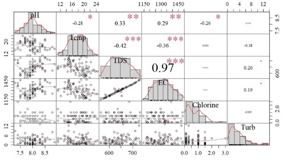
Figure 5, which is a correlation matrix, illustrates the relationship between the free chlorine residual (the target parameter) and the other water quality parameters (the predictor parameters) in the study area water supply network statistically. Based on the correlation matrix analysis, there is no significant correlation between chlorine and the other parameters except for pH. A weak but statistically significant negative correlation (Pearson coefficient = −0.26, confidence interval = [−0.455, −0.048], and p-value = 1.76 × 10⁻²) is observed between free chlorine residual and pH. Hence, there is statistical evidence that the relationship between the two parameters is meaningful (p < 0.05). Along the pH value range of 7.3–8.9, the reverse trend with the free chlorine residual is presented in Figure 6. Accordingly, moving to a higher pH level reduces the free chlorine concentration in the water due to the pH dependency. Chemically, this is due to the shifting of hypochlorous acid (HOCl) dissociation in water toward hypochlorite ions (OCl⁻) (Eqs. (4) and (5)) [41, 42]. As pH increases toward the upper observed limit (8.9), the balance shifts toward OCl⁻, which has significantly lower disinfection efficiency compared to HOCl.
Cl₂ + H₂O ⇌ HOCl + H⁺ + Cl⁻ (4)
HOCl ⇌ H⁺ + OCl⁻ (5)
Figure 5. Correlation matrix of the measured water quality parameters
Figure 6. The free chlorine residual and pH trend in the water supply network
Moreover, it is scientifically noted that the presence of chlorine residual can contribute to a slight decrease in the water pH levels, a finding that aligns with the observations of previous studies [12, 38, 43] regarding the acidic effect of chlorine species in water. This dual interaction explains the inverse correlation between these two parameters in the study area water supply network. However, the causality is not demonstrated because distance, water age, turbidity, pipe material, pipe age and hydraulic conditions were not controlled. Thus, although temperature, TDS, EC, and turbidity provide a reliable indication of the water quality characteristics, the chlorine-pH interaction is the key predictor of disinfection efficiency.
3.2 Mapping of the free chlorine residual spatial distribution
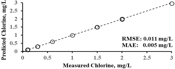
The free chlorine residual concentration at any location in the network essentially decreases with the distance from the chlorine source [5, 12, 30], which is the WTP reservoir here. Accordingly, the spatial distribution of the free chlorine residual concentrations and the pH levels was represented using the IDW interpolation method to display the change between the sampling locations in the water supply system, as shown in Figure 7(a). The maximum chlorine concentration is located at the WTP site and decreases with distance along the pipe network. Since the pH levels affect the free chlorine residual in the study area water supply network (Figures 5 and 6), the pH levels map in Figure 7(b) reflects this relationship spatially. The locations of high pH levels show low free chlorine residual concentrations. In order to prove the spatial distribution maps constructed by the IDW interpolation method, 28 additional sampling locations were independently assigned as validation locations. The measured free chlorine residual and pH from the validation locations were compared with the values predicted by the IDW method. Figures 8 and 9 depict the 28 validation measurements and the validation plots, respectively, indicating an excellent agreement between the measured and predicted values for both parameters. Results obtained demonstrated a RMSE value of 0.0110 mg/L and a MAE of 0.0050 mg/L for the free chlorine residual concentrations and a RMSE value of 0.0063 and a MAE of 0.0034 for the pH levels. This indicates that the spatial distribution maps over the study area water supply system have been successfully represented by the IDW method. The complete data set for the 28 validation sampling locations (geographic coordinates, measured values, and IDW predicted values) is included in Table A1 (Appendix).
In these central areas of Al-Hilla District, the locations situated along the network main lines or close to the WTP show higher chlorine concentrations (up to 3.0 mg/L) coinciding with the lower pH values. Conversely, as water travels toward the surrounding neighborhoods and far locations, a significant decline in chlorine concentration is observed. These variations in chlorine concentrations can probably be attributed to different interconnected factors, including the differences in distance between the water supply reservoir and the served areas. Hence, as all network pipelines are fed from the same source, chlorine concentration decreases as the travel distance through the distribution network increases along the network pipes [12, 44]. Similarly, hourly variations, hydraulic fluctuations, and reaction kinetics over time also increase or decrease the water age, which possibly enhances the variability of chlorine concentrations in the distribution network during low demand periods [11, 13]. In addition, network pipe degradation that takes place in network pipes over time, such as leakages, illegal joints, old pipes, or damaged pipes, may cause a reduction in chlorine concentrations. Moreover, when the chlorine dosage at the WTP is not efficient, it makes the concentration of chlorine lower.
Figure 7. The Inverse Distance Weighting (IDW) interpolation map of (a) free chlorine residual concentrations in mg/L and (b) pH levels over the study area
Figure 8. Boxplots of the measured water quality parameters at the 28 validation sampling locations
(a)
(b)
Figure 9. The Inverse Distance Weighting (IDW) interpolation map validation plot of (a) free chlorine residual concentrations and (b) pH levels over the study area
3.3 Mapping of the free chlorine residual compliance with the standards
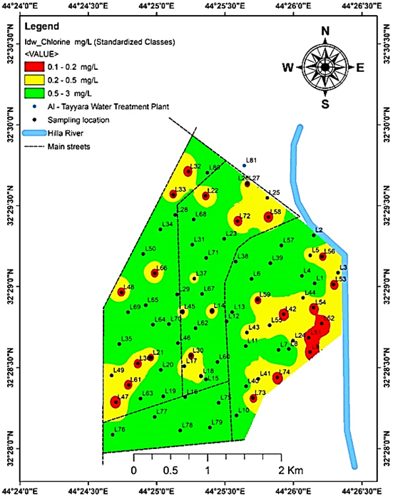
Within the free chlorine residual concentrations recorded range of 0.1–3.0 mg/L, the thresholds of standards, 0.2 and 0.5 mg/L, are chosen to categorize the chlorine concentrations distribution of tap water spatially. This way will zone regions where free chlorine residual concentrations failed or succeeded in meeting the standards, assessing the compliance throughout the water supply network. Accordingly, three interest zones (green, yellow, and red) were detected as depicted in Figure 10.
In the red zones, the free chlorine residual concentrations of tap water are below the Iraqi, WHO, and EPA minimum permissible limit of 0.2 mg/L (chlorine < 0.2 mg/L). Hence, values of 0.1 mg/L were reported at a significant portion of the 81 sampling locations (Figure 4). The 27 sampling points in this critical red zone represent 33.33% of the total 81 sampling points and show severe chlorine deficiency.
Notably, the red zones spread randomly over the study area, implying that the cause is not only due to chlorine decay with distance. These zones are largely located in old neighborhoods (Al-Souq, Abu Al-Qasim Street, Imam Ali Street, Bab Al-Hussein, and in parts of Hay Al-Hussein and Al-Jamiya) where older water distribution pipes exist, resulting in additional chlorine requirement because of system corrosion, biofilm growth, and sediment issues [45]. Additionally, locations of high turbidity, such as Hay Al-Hussein (13.6 NTU) and Al-Jamiya (7.7 NTU), probably contributed to the increase in chlorine demand and lowering the free chlorine residual concentrations [46]. World Health Organization [3] recommended dosing with free chlorine of about 2 mg/L to clear water (turbidity < 10 NTU) and 4 mg/L to turbid water (turbidity > 10 NTU). Dhanabal and Chellaiah [4] confirmed that the presence of low free chlorine residual in some neighborhoods is probably due to a combination of factors other than just distance from the WTP, including old infrastructure, high chlorine demand, and local hydraulic conditions. These zones, however, contain some low free residual chlorine, which provides a potential indicator of a lower level of protection against pathogen disinfection in these locations, and suggests a need to implement targeted infrastructure upgrades, operational investigations and subsequent microbiological monitoring to ensure safe water supplies throughout the network.
On the other hand, both yellow and green zones met the three standards (chlorine ≥ 0.2 mg/L). For the yellow zones. the tap water chlorine concentrations met the minimum requirement of the standards. Hence, 11 out of 81 sampling locations were recorded with a free chlorine residual concentration of 0.3 mg/L. However, these zones are very close to the standard threshold (0.2 mg/L). The yellow zones need continuous monitoring to ensure good disinfection efficiency. Compared with guidelines, these zones have low-risk scenarios. With increased epidemic risks, higher dosage is necessary to achieve greater disinfection efficacy. Thus, it should be noted that an initial dose of chlorine at the WTP reservoir is cautiously adjusted to prevent free chlorine residual losses. For the green zone, a good agreement with the standards was achieved. The free chlorine residual concentrations were as high as 3.0 mg/L in this zone. The high free chlorine residual recorded in these locations could be related to the good hydraulic conditions encountered along the main pipelines where water flows continuously and may have a short residence time, thereby minimizing chlorine decay. For instance, neighborhoods such as Al-Karama, Hay Shubber, Al-Iskan, 40th Street, and Al-Qiyada Street include locations of main roads and more recent residential developments. Also, the relatively new distribution system in some residential areas can decrease chlorine demand as a result of decreased pipe corrosion, sediment buildup, and biofilm growth, which can help ensure there is free chlorine residual in the distribution system within recommended levels [45, 47].
Furthermore, dosage determination strongly depends on turbidity. For low turbidity waters of less than 10 NTU, a standard fixed dose of approximately 2.0 mg/L is adequate, but for high turbidity waters of 10 to 100 NTU, one to two times higher baseline dosages of 4.0 to 5.0 mg/L are necessary since the chlorine demand increases significantly with suspended particles at the higher dissolved organic matter concentrations [48, 49]. As a result, dosing at the source must be high enough to guarantee reassuring residual coverage across the water distribution network and through domestic storage for days of 8 to 24 hours or more [50]. However, operational methods must be strictly bounded by the upper thresholds of standards, 4.0 or 5.0 mg/L, carefully avoiding unacceptably off-taste and odor in tap water [49].
In general, 14 (17.28%) of the sampling points were above the maximum permissible turbidity limit of 5.0 NTU and 4 (4.94%) points were above the upper limit of the pH range (>8.5).
3.4 Design implications and spatial decision support
The spatial mapping of free chlorine residual extends beyond a diagnostic water quality assessment. It serves as a foundational spatial design tool for engineering layout optimization and structural risk mitigation within the water supply infrastructure. By translating raw concentration data into a map of free chlorine residual compliance with standards, this study establishes a spatial decision support framework that bridges the gap between water quality data and infrastructure management. Specifically, the generated maps identify structural weakness zones that include areas characterized by accelerated chlorine standards violations (highlighted in red in Figure 10), allowing municipal planners to strategically optimize the design of monitoring layouts and secondary booster chlorination stations. Rather than relying on a uniform, resource-intensive monitoring approach, utilities can utilize these spatial models to design an adaptive, risk-prioritized network. This design application ensures that regulatory interventions and infrastructure upgrades are targeted precisely at locations that fail drinking-water standards, thereby reinforcing the environmental resilience and biosafety of the entire distribution network.
Figure 10. Spatial distribution of free chlorine residual in mg/L over the study area based on the standard limits
The spatial distribution of free chlorine residual in tap water in a central region of Al-Hilla District, Iraq, has been explored by analyzing different interactions in the water supply network. Correlation analysis based on the measured water quality parameters (pH, temperature, TDS, EC, turbidity, and free chlorine residual) has identified a statistically significant inverse relationship between the free chlorine residual and pH. Hence, a linear trend is recognized between them. Comparisons with the Iraqi, WHO, and EPA standards revealed turbidity and free chlorine residual violations. In the present local district, the findings also showed that mapping the free chlorine residual concentrations and pH levels using the IDW interpolation method revealed spatial zones in which the high free chlorine residual concentration zone has low pH levels, confirming the statistically significant correlation. In addition, the free chlorine residual violated the standards at the study area network locations where the distance to the WTP site is far. However, other possible influences can interact with the distance effect, including turbidity issues, leakages, illegal joints, old pipes, or damaged pipes, reducing the free chlorine residual concentrations. Thus, it is required to improve the water supply network infrastructure in the study area. From this single short sampling campaign in the local study area, chlorine dosage at the WTP helps boost the disinfection efficiency at the tap water locations. However, the dosage strategy must be heavily adjusted and carefully evaluated against inherent trade-offs. Any increase in dosage must be evaluated for by-products such as DBP formation, compliance with standards, and taste-and-odor thresholds. Finally, the IDW interpolation method is a powerful GIS tool for producing visual representations of spatial variability in the free chlorine residual across networks, identifying problem areas and supporting future monitoring and management strategies.
Table A1. Geographic location, measured and IDW-predicted values of free chlorine and pH at the 28 validation sites
|
Sample Number |
Coordinates |
Measured Value Cl |
Predicted Value Cl |
Measured Value pH |
Predicted Value pH |
|
|
Latitude (°N) |
Longitude (°E) |
|||||
|
V1 |
32.48015702 |
44.43749083 |
0.1 |
0.102461 |
8.2 |
8.196839 |
|
V2 |
32.48471868 |
44.43764372 |
0.1 |
0.111893 |
8.3 |
8.299078 |
|
V3 |
32.48803228 |
44.43372343 |
2.0 |
1.996289 |
7.8 |
7.801105 |
|
V4 |
32.47697083 |
44.43147188 |
1.5 |
1.497043 |
7.7 |
7.702258 |
|
V5 |
32.47562425 |
44.42665745 |
1.5 |
1.495509 |
7.8 |
7.801975 |
|
V6 |
32.47305968 |
44.42699238 |
0.1 |
0.100812 |
7.5 |
7.518405 |
|
V7 |
32.47043715 |
44.42176292 |
1.5 |
1.49895 |
7.5 |
7.501225 |
|
V8 |
32.48530687 |
44.4264596 |
0.1 |
0.100263 |
7.7 |
7.704587 |
|
V9 |
32.48087357 |
44.42749402 |
1.0 |
1.000007 |
8.3 |
8.299364 |
|
V10 |
32.48231463 |
44.41523308 |
0.3 |
0.300328 |
8.5 |
8.500177 |
|
V11 |
32.4697445 |
44.4127039 |
1.5 |
1.497729 |
8.5 |
8.500396 |
|
V12 |
32.47121422 |
44.41873573 |
0.1 |
0.10118 |
8.5 |
8.497416 |
|
V13 |
32.47339857 |
44.42478352 |
1.5 |
1.497729 |
8.4 |
8.396005 |
|
V14 |
32.47388937 |
44.42005503 |
2.0 |
1.97339 |
8.5 |
8.495074 |
|
V15 |
32.48063727 |
44.41905578 |
0.1 |
0.111509 |
8.8 |
8.799099 |
|
V16 |
32.4921834 |
44.42964522 |
1.5 |
1.493447 |
8.8 |
8.799335 |
|
V17 |
32.49227193 |
44.42735893 |
0.1 |
0.108631 |
8.5 |
8.485306 |
|
V18 |
32.49474473 |
44.42742132 |
3.0 |
2.951149 |
7.4 |
7.421483 |
|
V19 |
32.47055088 |
44.41130782 |
0.1 |
0.104891 |
8.8 |
8.798883 |
|
V20 |
32.48056445 |
44.42450437 |
1.5 |
1.498775 |
8.7 |
8.699177 |
|
V21 |
32.48424358 |
44.42322442 |
0.6 |
0.599716 |
8.5 |
8.499105 |
|
V22 |
32.48809127 |
44.42771107 |
0.3 |
0.302636 |
7.9 |
7.901026 |
|
V23 |
32.47549188 |
44.43494343 |
1.5 |
1.497511 |
8.2 |
8.197033 |
|
V24 |
32.48409905 |
44.43578205 |
1.5 |
1.498029 |
8.0 |
8.000395 |
|
V25 |
32.4770126 |
44.41678838 |
2.0 |
1.999115 |
8.8 |
8.797833 |
|
V26 |
32.48203132 |
44.4171531 |
0.1 |
0.100107 |
8.5 |
8.500021 |
|
V27 |
32.4884696 |
44.41735562 |
0.1 |
0.100088 |
8.2 |
8.200285 |
|
V28 |
32.48747062 |
44.41442205 |
0.3 |
0.299976 |
8.1 |
8.101186 |
Note: Inverse Distance Weighting (IDW); Chlorine (Cl).
[1] Li, P., Wu, J. (2019). Drinking water quality and public health. Exposure and Health, 11(2): 73-79. https://doi.org/10.1007/s12403-019-00299-8
[2] Gudeta, B., Ratnam, M.V., Mohan, R. (2022). Physiochemical analysis of drinking water and treatment with a homemade filter: A case study of Illu Abba Bor Zone, Ethiopia. International Journal of Analytical Chemistry, 2022(1): 4333938. https://doi.org/10.1155/2022/4333938
[3] World Health Organization. (2022). Guidelines for drinking-water quality: Fourth edition incorporating the first and second addenda. World Health Organization, Switzerland. https://www.who.int/publications/i/item/9789240045064.
[4] Dhanabal, G., Chellaiah, G. (2025). Enhancing residual chlorine stability in water distribution systems: Challenges, modeling approaches, and advanced optimization strategies. Next Chemical Engineering, 1: 100005. https://doi.org/10.1016/j.nxcen.2025.100005
[5] Onyutha, C. (2024). Influence of physical and water quality parameters on residual chlorine decay in water distribution network. Heliyon, 10(10): e30892. https://doi.org/10.1016/j.heliyon.2024.e30892
[6] Beshir, A., Reddythota, D., Alemayehu, E. (2024). Evaluation of drinking water quality and associated health risks in Adama City, Ethiopia. Heliyon, 10(16): e36363. https://doi.org/10.1016/j.heliyon.2024.e36363
[7] Fisher, I., Kastl, G., Sathasivan, A. (2023). Validity of chlorine-wall reaction models for drinking water distribution systems. Urban Water Journal, 20(9): 1157-1168. https://doi.org/10.1080/1573062X.2023.2241437
[8] Obaid, S., Hosoi, K., Ngoc, N.M., Inoue, T., Yokota, K. (2025). Modelling free residual chlorine decay in a residential district water distribution network using smart water meter data. International Journal of Environmental Science and Technology, 22(12): 11809-11816. https://doi.org/10.1007/s13762-025-06378-5
[9] Khor, Y., Aziz, A.A., Chong, S.S. (2024). Recent developments and sustainability in monitoring chlorine residuals for water quality control: A critical review. RSC Sustainability, 2(9): 2468-2485. https://doi.org/10.1039/d4su00188e
[10] Monteiro, L., Figueiredo, D., Dias, S., et al. (2014). Modeling of chlorine decay in drinking water supply systems using EPANET MSX. Procedia Engineering, 70: 1192-1200. https://doi.org/10.1016/j.proeng.2014.02.132
[11] Kulmedov, B., Eroglu, E., Kandymov, N. (2025). Modeling the factors affecting residual chlorine decay in the water distribution network of Abuja, Nigeria. Water Quality Research Journal, 60(3): 482-497. https://doi.org/10.2166/wqrj.2025.006
[12] Bahrudin, M., Yulistyorini, A., Rahayuningsih, T. (2022). Analysis of residual chlorine concentration in distribution network of drinking water supply at Istana Dieng II Residence of Malang, East Java, Indonesia. Indonesian Journal of Urban and Environmental Technology, 5: 223-239. https://doi.org/10.25105/urbanenvirotech.v5i3.12463
[13] Yousefi, M., Mesbahi, F., Abbasi, I., Kousha, M., Rahmani, K. (2020). Application of geographical information system (GIS) in analysis and detection of microbial contamination in water supply network. Journal of Health Sciences and Surveillance System, 8(3): 110-114. https://doi.org/10.30476/jhsss.2020.86434.1091
[14] Mohammadi, A., Miri, M., Ebrahimi, A., Khorsandi, H., Nemati, S. (2016). Monitoring of THMs concentration in Isfahan water distribution system and zoning by GIS, a case study in the center of Iran. Iranian Journal of Health, Safety and Environment, 3(1): 421-427.
[15] Arslan, O., Bagdatlı, C.M. (2025). GIS-based mapping and spatial modeling of drinking water quality in the capital city of Turkiye. Rocznik Ochrona Środowiska, 27: 229-239. https://doi.org/10.54740/ros.2025.019
[16] Al-Zubaidi, H.A.M., Kadhim, E.J., Jasim, H.K., Naje, A.S., Al-Jassani, F.D., Chelliapan, S. (2025). Machine learning analysis for the Hilla River water quality index-Iraq. Global NEST Journal, 27(3): 1-8. https://doi.org/10.30955/gnj.06980
[17] Al-Jassani, F.D., Al-Zubaidi, H.A., Al-Mansori, N.J. (2022). Satellite-based statistical analysis of Hilla River water quality parameters, Iraq. Nature Environment and Pollution Technology, 21(5): 2315-2321. https://doi.org/10.46488/NEPT.2022.v21i05.027
[18] U.S. Geological Survey. (2015). National field manual for the collection of water-quality data. U.S. Geological Survey. https://doi.org/10.3133/twri09
[19] U.S. Environmental Protection Agency. (1979). Handbook for analytical quality control in water and wastewater laboratories (EPA-600/4-79-019). EPA Office of Research and Development. https://www.epa.gov/sites/default/files/2015-06/documents/QCHandbook.pdf.
[20] Al Yousif, M.A., Maytham, K.O., Al-Zubaidi, H.A., et al. (2025). A simplified strategy for evaluating the performance of water treatment plants. Ecological Engineering and Environmental Technology, 26(10): 26-35. https://doi.org/10.12912/27197050/209743
[21] Abbas, H.A. (2025). Iraqi drinking water quality standards (IQS417/2009)-revisited. Tikrit Journal of Engineering Sciences, 32(1): 1606. https://doi.org/10.25130/tjes.32.1.23
[22] Al-Mayah, W.T., Al-Tmemy, W.B. (2024). Efficiency of treatment plant and drinking water quality assessment in Al-Numaniyah City, Iraq. In 6th International Conference of Modern Technologies in Agricultural Sciences, Kufa, Najaf, Iraq, pp. 527-537.
[23] Al-Mousawey, H.J., Abed, B. (2023). Water quality assessment of Al-Najaf City potable water network. Journal of Engineering, 29(4): 14-29. https://doi.org/10.31026/j.eng.2023.04.02
[24] Al-Mayah, W.T. (2021). Evaluation of efficiency of drinking water treatment plant in Al-Aziziyah City, Iraq. Scientific Research Journal of Agriculture and Life Sciences, 2(2): 1-8.
[25] Agudelo-Vera, C., Avvedimento, S., Boxall, J., et al. (2020). Drinking water temperature around the globe: Understanding, policies, challenges and opportunities. Water, 12(4): 1049. https://doi.org/10.3390/W12041049
[26] Naghipour, D., Ashrafi, S.D., Mojtahedi, A., Vatandoost, M., Hosseinzadeh, L., Roohbakhsh, E. (2017). Data on microbial and physiochemical characteristics of inlet and outlet water from household water treatment devices in Rasht, Iran. Data in Brief, 16: 1005. https://doi.org/10.1016/j.dib.2017.12.038
[27] World Health Organization. (2021). A global overview of national regulations and standards for drinking-water quality. World Health Organization, Switzerland. https://www.who.int/publications/i/item/9789240023642.
[28] Susatio, R., Riyanto, I.A., Wilopo, W., Hendrayana, H. (2025). Comparative evaluation of IDW and spline interpolation methods for analyzing groundwater table depth and elevation. Jurnal Ilmiah Dinamika Rekayasa, 21(2): 98-106.
[29] Jasim, A.K., Walli, H.A. (2023). Analysis of hotspots and inverse distance weighting (IDW) of polluted habitats using ArcGIS Pro: A case study in the sea of Najaf and surrounding terrestrial area. IOP Conference Series: Earth and Environmental Science, 1215(1): 012005. https://doi.org/10.1088/1755-1315/1215/1/012005
[30] Ajaj, Q.M., Shareef, M.A., Hassan, N.D., Hasan, S.F., Noori, A.M. (2018). GIS based spatial modeling to mapping and estimation relative risk of different diseases using inverse distance weighting (IDW) interpolation algorithm and evidential belief function (EBF) (Case study: Minor part of Kirkuk City, Iraq). International Journal of Engineering and Technology, 7(4): 185-191.
[31] Setianto, A., Triandini, T. (2013). Comparison of kriging and inverse distance weighted (IDW) interpolation methods in lineament extraction and analysis. Journal of Applied Geology, 5(1): 21-29. https://doi.org/10.22146/jag.7204
[32] Hua, A.K., Baharudin, M.N., Ngadiran, S.N.A., Sulaiman, S. (2025). Integrated principal component analysis (PCA) and inverse distance weighted (IDW) modeling for water quality assessment in the Melaka River Basin. Applied Ecology and Environmental Research, 23(5): 10315-10332. https://doi.org/10.15666/aeer/2305_1031510332
[33] Prasood, S.P., Mukesh, M.V., Sajinkumar, K.S., Thrivikramji, K.P. (2023). COVID-19 pandemic lockdown modulation of physico-chemical parameters of surface water, Karamana river basin, Southwest India: A weighted arithmetic index and geostatistical perspective. Total Environment Research Themes, 6: 100042. https://doi.org/10.1016/j.totert.2023.100042
[34] Yasin, K.H., Gelete, T.B., Iguala, A.D., Kebede, E. (2024). Optimal interpolation approach for groundwater depth estimation. MethodsX, 13: 102916. https://doi.org/10.1016/j.mex.2024.102916
[35] Dimitriadou, S., Nikolakopoulos, K.G. (2022). Development of the statistical errors raster toolbox with six automated models for raster analysis in GIS environments. Remote Sensing, 14(21): 5446. https://doi.org/10.3390/rs14215446
[36] Al-Zubaidi, H.A., Wells, S.A. (2020). Analytical and field verification of a 3D hydrodynamic and water quality numerical scheme based on the 2D formulation in CE-QUAL-W2. Journal of Hydraulic Research, 58(1): 152-171. https://doi.org/10.1080/00221686.2018.1499051
[37] Chai, T., Draxler, R.R. (2014). Root mean square error (RMSE) or mean absolute error (MAE)?–Arguments against avoiding RMSE in the literature. Geoscientific Model Development, 7(3): 1247-1250. https://doi.org/10.5194/gmd-7-1247-2014
[38] Abbas, A.H. (2011). Studying of residual chlorine concentration within water supply distribution system in Samarra City-Iraq. International Review of Chemical Engineering, 3(5): 622-626.
[39] Amogne, A.A. (2026). Spatial and temporal analysis of drinking water quality using GIS-based geostatistical techniques. Discover Hazards, 2: 41. https://doi.org/10.1007/s44475-026-00045-0
[40] Mahmood, Y.H. (2018). Concentration of residual chlorine and its health effects in the drinking water of the Kirkuk City. Kafkas Üniversitesi Fen Bilimleri Enstitüsü Dergisi, 11(1): 29-37.
[41] Mehendale, F.V., Clayton, G., Homyer, K., Reynolds, D.M. (2023). HOCl vs OCl−: Clarification on chlorine-based disinfectants used within clinical settings. Journal of Global Health Reports, 7: e2023052. https://doi.org/10.29392/001c.84488
[42] Onyutha, C., Kwio-Tamale, J.C. (2022). Modelling chlorine residuals in drinking water: A review. International Journal of Environmental Science and Technology, 19(11): 11613-11630. https://doi.org/10.1007/s13762-022-03924-3
[43] Choi, Y., Byun, S.H., Jang, H.J., Kim, S.E., Choi, Y.J. (2022). Comparison of disinfectants for drinking water: Chlorine gas vs. on-site generated chlorine. Environmental Engineering Research, 27(1): 200543. https://doi.org/10.4491/eer.2020.543
[44] Baker, B.R. (2016). The effect of a distance from water treatment plant on residual chlorine. International Journal of Advanced Engineering Research and Science, 3(10): 181-186. https://doi.org/10.22161/ijaers/3.10.29
[45] Zhou, Q., Bian, Z., Yang, D., Fu, L. (2023). Stability of drinking water distribution systems and control of disinfection by-products. Toxics, 11(7): 606. https://doi.org/10.3390/toxics11070606
[46] Molina-Pinna, J., Román-Velázquez, F.R. (2025). The bactericide effects of chitosan when used as an indicator of chlorine demand. Polymers, 17(9): 1226. https://doi.org/10.3390/polym17091226
[47] Absalan, F., Hatam, F., Barbeau, B., Prévost, M., Bichai, F. (2022). Predicting chlorine and trihalomethanes in a full-scale water distribution system under changing operating conditions. Water, 14(22): 3685. https://doi.org/10.3390/w14223685
[48] Gallandat, K., Stack, D., String, G., Lantagne, D. (2019). Residual maintenance using sodium hypochlorite, sodium dichloroisocyanurate, and chlorine dioxide in laboratory waters of varying turbidity. Water, 11(6): 1309. https://doi.org/10.3390/w11061309
[49] Branz, A., Levine, M., Lehmann, L., et al. (2017). Chlorination of drinking water in emergencies: A review of knowledge to develop recommendations for implementation and research needed. Waterlines, 36(1): 4-39. https://doi.org/10.3362/1756-3488.2017.002
[50] Ali, S.I., Ali, S.S., Fesselet, J.F. (2020). Evidence-based chlorination targets for household water safety in humanitarian settings: Recommendations from a multi-site study in refugee camps in South Sudan, Jordan, and Rwanda. Water Research, 189: 116642. https://doi.org/10.1016/j.watres.2020.116642