Comparative Estimation and Spatial Distribution Mapping of Total Suspended Solids Using Four Empirical Algorithms and Sentinel-2 Level-2A Imagery in the Downstream Krueng Aceh Watershed, Indonesia: A Single-Date Assessment in 2025

Water quality reflects the condition of a water body and its suitability for supporting human needs and ecosystem sustainability. In general, water quality parameters are grouped into three main categories, namely physical, chemical, and biological parameters, each of which plays an important role in assessing the characteristics and ecological functions of water bodies [1].

TSS is an important parameter that is used to assess water quality by indicating the concentration of suspended particles. In the past couple of decades, remote sensing has become a key tool for comprehensive environmental monitoring. The use of satellite imagery enables broad spatial observation and continuous analysis of environmental parameters, which is particularly important in coastal and estuarine areas. One of the most widely used remote sensing systems is Sentinel-2. This satellite provides multispectral data with high spatial resolution (up to 10 meters in some bands). Sentinel-2 captures the light spectrum from visible to near-infrared, which is highly sensitive to changes in suspended particle content in water [2].

Human activities along the Krueng Aceh watershed area, such as agriculture, settlement, and infrastructure development, have worsened the sedimentation and water turbidity problem. This reduces water clarity, inhibits light penetration for photosynthesis by aquatic organisms, and accelerates river siltation. Downstream areas such as the Krueng Aceh estuary are vulnerable to flooding and water quality degradation, especially in areas adjacent to markets and landfills [3]. Increasing population growth leads to higher water resource demand, highlighting the importance of water resource management that considers environmental carrying capacity [4]. In addition to land-use and urban activities, wastewater and leachate inputs may also contribute to local variations in water quality. Previous monitoring at the Blang Bintang landfill reported a decline in water quality in the Krueng Uteun Siblah River immediately downstream of the leachate outfall, with increased BOD, COD, and Fe concentrations and decreased dissolved oxygen levels [5].

Remote sensing offers substantial advantages over traditional monitoring methods, especially due to the synoptic coverage and temporal consistency of the data, and has the potential to provide important information about inland transitional waters and near coastal areas [6]. Satellite remote sensing technology is widely used to monitor and detect the dynamic changes in water quality parameters. This approach offers broad spatial and temporal coverage by utilizing various satellite sensors operating at visible and infrared wavelengths, enabling continuous and comprehensive observation of water conditions [7].

Sentinel-2A is capable of providing continuous and high-quality data that is highly supportive in providing water quality information through the Multi Spectral Imager (MSI) sensor. TSS can be estimated based on algorithms developed by Laili et al. [8], Budhiman [9], Liu et al. [10], and Parwati and Purwanto [11] from Sentinel-2A images. Therefore, the purpose of this study is to compare the accuracy of several algorithms using Sentinel-2A images with laboratory test results so that water quality evaluation can be identified quickly.

Although Sentinel-2 has been widely used for TSS estimation, the performance of empirical algorithms may vary among different water bodies because of differences in optical properties, suspended sediment characteristics, and local environmental conditions. Therefore, an algorithm developed and validated in one river, lake, or coastal environment may not provide similar accuracy when transferred to another region. In the downstream Krueng Aceh watershed, this issue is particularly relevant because the water environment is influenced by riverine processes, sediment transport, and anthropogenic activities. Therefore, this study compares four previously developed empirical TSS algorithms, namely Laili, Liu, Budhiman, and Parwati, using Sentinel-2 Level-2A imagery and laboratory-measured TSS data. The novelty of this study lies in evaluating the relative performance, regional suitability, and transferability of existing algorithms under the optical conditions of downstream Krueng Aceh, rather than developing a new TSS retrieval model. Accordingly, this study aims to identify which existing empirical algorithm provides the most suitable performance for TSS estimation in the study area.

One of the limitations in the application of remote sensing lies in the variation in spatial, temporal, and spectral resolution of the sensors used in the data acquisition process. Sensors with long re-recording intervals tend to have limitations in detecting the temporal dynamics of water quality parameters, such as TDS and TSS. Each satellite sensor has different resolution characteristics in terms of spatial, spectral, and temporal aspects. For example, Landsat 8 OLI has a revisit period of approximately 16 days, while Sentinel-2A/B MSI offers a shorter interval of approximately 5 days, making it more optimal for detecting temporal changes in water quality [12, 13].

The results of TSS measurements through laboratory tests from 10 sampling points in the Krueng Aceh Hilir watershed are presented in Table 1. Samples were taken at geographically dispersed locations with longitude coordinates varying from 95°18'53" E to 95°21'44" E and latitude coordinates varying from 5°30'34" N to 5°34'57" N. The laboratory test data showed variations in TSS values among the ten sampling points and were used as observed TSS values for evaluating the performance of the empirical algorithms. Because no independent test dataset was available, model performance was assessed using LOOCV.

The ten sampling points represented different downstream settings with varying levels of anthropogenic activity. Points 1-4 were located in the Lambaro area, which includes market activities, water-treatment infrastructure, agricultural areas, livestock activities, and river infrastructure. Points 5-9 were located in the urban area of Banda Aceh, characterized by dense settlements, bridges, commercial activities, and boat-mooring areas. Point 10 was located near the river mouth, close to the coastal zone.

The highest laboratory-measured TSS concentration was observed at Point 1 (11.3 mg/L), followed by Point 5 (10.5 mg/L), Point 9 (9.6 mg/L), and Point 8 (9.2 mg/L). The relatively high TSS concentration at Point 1 may be associated with intensive activities around Lambaro Market, although this relationship was not directly tested because land-use intensity, rainfall, and runoff were not measured. The TSS concentration at Point 2 was lower (6.9 mg/L), which may reflect differences in local environmental conditions and anthropogenic activities around the water-treatment facility. Point 3 recorded 7.1 mg/L, while Point 4 recorded 8.5 mg/L; the observed variation may be related to local flow conditions, sedimentation, and surrounding agricultural and livestock activities. However, these factors were not directly measured in this study and therefore cannot be confirmed as causes of the observed TSS differences.

Points 5-9 showed spatial variability in TSS concentrations within the urban downstream section. Point 5 recorded 10.5 mg/L, which may be associated with the surrounding dense settlement and urban drainage network. Point 6 recorded 9.0 mg/L, whereas Point 7 recorded 7.1 mg/L, indicating local differences in TSS conditions despite their urban setting. Point 8 recorded 9.2 mg/L and was located in an area with dense settlements and commercial activities. Point 9 recorded 9.6 mg/L near the boat-mooring area in Kampung Jawa. Vessel activity and sediment disturbance may be possible explanations for the relatively high TSS value at this location; however, vessel traffic was not measured during sampling.

The lowest TSS concentration was observed at Point 10 (6.4 mg/L), located near the river mouth. This relatively low value may be associated with mixing between river and seawater and tidal dynamics; however, tidal conditions, river discharge, and rainfall were not measured during the survey. Therefore, these factors should be considered possible explanations rather than demonstrated causes.

Estimation of TSS concentrations obtained from Sentinel-2 Level-2A image processing using four estimation algorithms, namely Laili et al. [8], Budhiman [9], Liu et al. [10], and Parwati and Purwanto [11], at each sampling location is presented in Table 2. The results illustrate spatial variation in TSS estimates and differences among the four algorithms at the same sampling locations. These values were compared with laboratory measurements to evaluate the performance of each image-based estimation method.

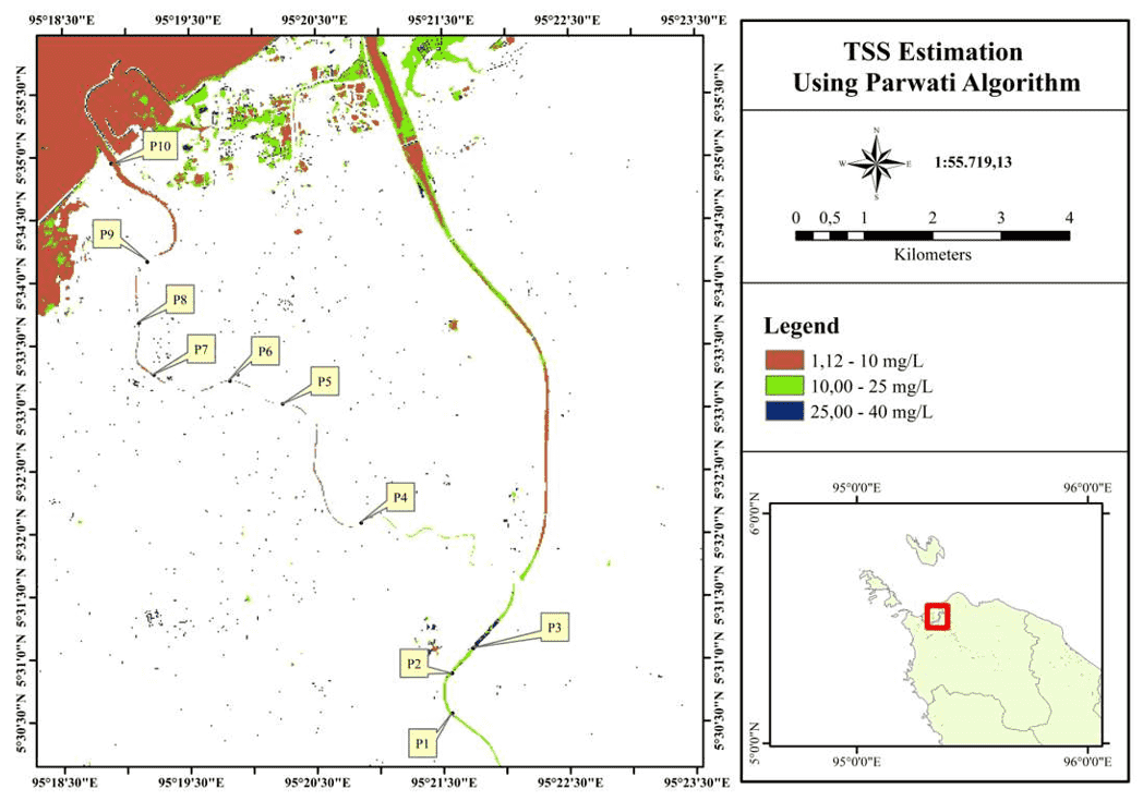
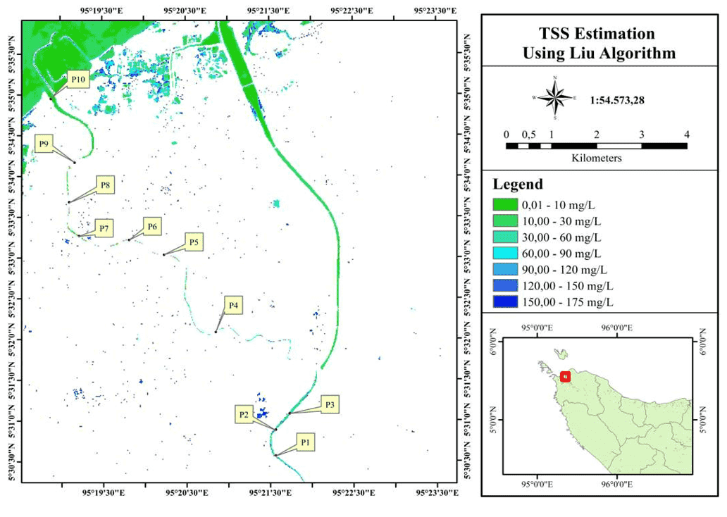
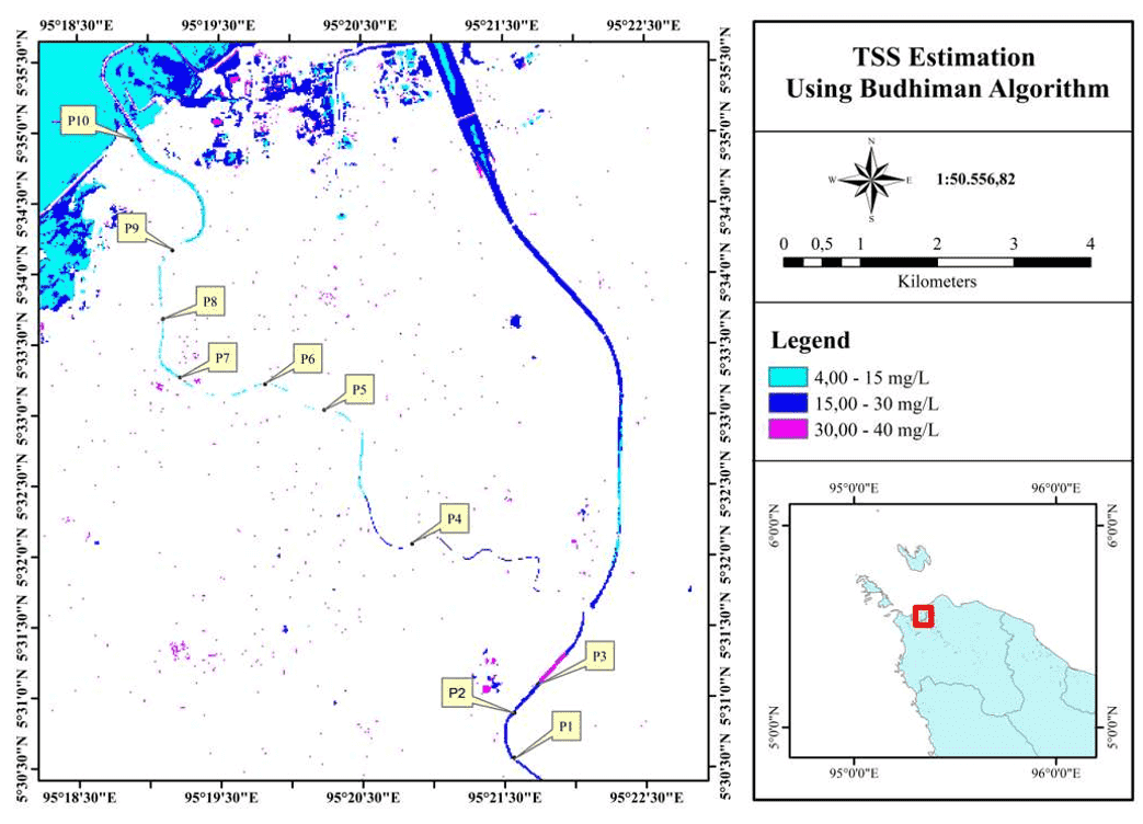
The estimation of TSS values using Sentinel-2 Level 2A imagery produced significant variations in values between the four algorithms applied (Figure 2). A comparative analysis reveals quite striking estimation disparities, with the Liu algorithm showing a tendency for high estimates at certain locations, particularly sampling location points 4 and 5, which reached 86.33 mg/L and 64.68 mg/L. These high values indicate that the Liu algorithm is highly sensitive to changes in reflectance in the red and near-infrared bands used in its calculations, enabling it to detect significant increases in suspended material in more turbid waters. On the other hand, lower values such as at location 6 (8.39 mg/L), location 8 (8.30 mg/L), and location 9 (10.33 mg/L) demonstrate the algorithm’s ability to capture spatial variations between high and low TSS areas. The average TSS value in Liu’s algorithm was at a medium to high level, indicating that this model tends to overestimate areas with high reflectance due to the presence of suspended materials and other optical elements such as phytoplankton or organic matter.

Table 2. Total Suspended Solids (TSS) measurement data from Sentinel-2 Level-2A

The Laili’s algorithm shows relatively stable TSS estimates, with values ranging from 15.03 to 19.79 mg/L. The highest recorded value was at location 1, with 19.79 mg/L, while the lowest value was at location 10, with 15.03 mg/L. The values at the other locations also showed relatively small variations, indicating the stability of the model in estimating TSS concentration. The consistency of these values indicates that Laili’s algorithm has moderate sensitivity to changes in water spectral characteristics, which is likely due to the use of interband ratios in the model formulation, thereby reducing the influence of reflectance anomalies and non-sediment materials.

The Budhiman’s algorithm estimates TSS concentrations ranging from 11.68 to 40.86 mg/L, with the maximum value observed at location 5 (40.86 mg/L) and the minimum value at location 7 (11.68 mg/L). Location 2 (28.48 mg/L) and location 3 (27.73 mg/L) also showed relatively high TSS values, indicating higher concentrations of suspended solids at these sampling locations. Parwati’s algorithm produced TSS estimates ranging from 5.77 to 39.24 mg/L, with the highest value recorded at location 5 (39.24 mg/L) and the lowest value at location 7 (5.77 mg/L). At several locations, particularly location 6 (6.01 mg/L), location 7 (5.77 mg/L), location 8 (6.52 mg/L), and location 9 (6.31 mg/L), the estimates showed relatively low values with narrow variability, indicating the stability of the algorithm’s estimates under low TSS conditions.

To assess the stability of the observed relationships between laboratory-measured TSS and the estimates generated by the four published algorithms under the limited sample size, the non-cross-validated results were compared with the LOOCV results (Table 3). Because the algorithms were applied using their original fixed coefficients, LOOCV was used as a performance-stability assessment rather than as a recalibration procedure.

Table 3. Comparison of non-cross-validated and leave-one-out cross-validation (LOOCV) performance of the four empirical Total Suspended Solids (TSS) algorithms

The results show a substantial difference between the non-cross-validated and LOOCV performance. Under LOOCV, the Laili algorithm produced the lowest RMSE (1.5163 mg/L) and MAPE (16.1822%) among the four algorithms, whereas the Liu algorithm produced the highest R² (0.1126). However, the R² value for Laili was only 0.0670, indicating limited predictive ability for the available observations. Liu also showed a low R² of 0.1126, while Budhiman and Parwati produced negative R² values of -0.5376 and -0.3084, respectively. Thus, although Laili showed the best relative performance among the four algorithms under LOOCV, its predictive ability remained weak.

The non-cross-validated results showed apparently better performance, particularly for Laili, with RMSE = 0.9799 mg/L, MAPE = 10.9420%, and R² = 0.6103. These statistics were calculated from the complete set of observations and may therefore provide an optimistic representation of the observed algorithm–field-data relationship under the small-sample condition. In contrast, the lower LOOCV performance indicates that this relationship was not stable when individual observations were sequentially excluded from the regression assessment. Therefore, the LOOCV results are considered the primary indicators for assessing performance stability in this study. The findings should be regarded as preliminary, and larger multi-season datasets with independent validation are required for a more robust assessment of the four published algorithms.

1.png

2.png

3.png

4.png

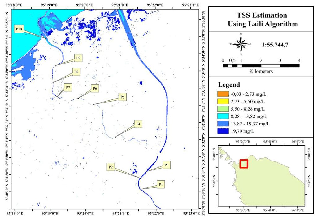
Figure 2. Total Suspended Solids (TSS) estimation results using several different algorithms

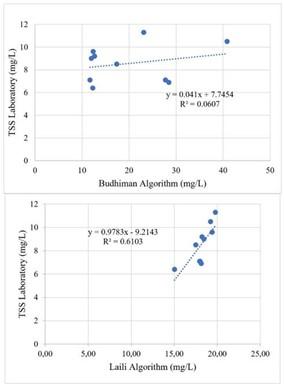
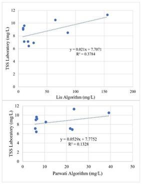
The comparison between in-situ measurements and the estimation results using satellite imagery was tested using a regression model. The relationship between parameter values can be seen in Figure 3.

The non-cross-validated (No CV) regression statistics are presented in Table 4 to provide a descriptive comparison of the relationships between laboratory-measured TSS and the estimates generated by the four algorithms. Laili showed the lowest non-cross-validated RMSE (0.9799 mg/L), MAE (0.8661 mg/L), and MAPE (10.94%), with an R² of 0.6103. However, these statistics should be interpreted only as descriptive, non-cross-validated results because they do not account for the stability of the regression relationship under the limited sample size. The corresponding LOOCV results provide a more conservative assessment and indicate substantially lower predictive performance, particularly for Laili (R² = 0.0670). Therefore, the non-cross-validated statistics are not used as the primary basis for ranking the algorithms.

3-1.jpg

3-2.jpg

Figure 3. Linear regression analysis results for the algorithm

Table 4. Non-cross-validated (No CV) regression statistics of the four empirical Total Suspended Solids (TSS) algorithms

4._jpg.jpeg

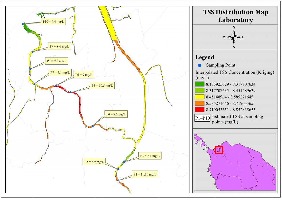
Figure 4. Ordinary Kriging-based interpolated spatial distribution of laboratory-measured Total Suspended Solids (TSS) and observed sampling points in the downstream Krueng Aceh watershed

5.jpg

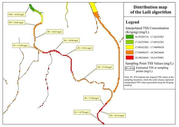
Figure 5. Spatial distribution of Total Suspended Solids (TSS) estimated using the Laili et al. [8] algorithm in the downstream Krueng Aceh watershed

6.jpg

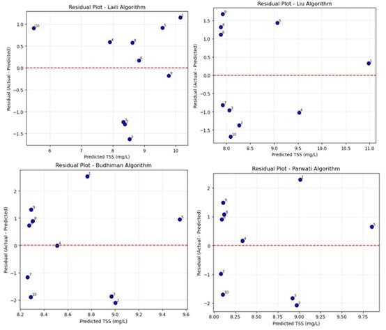
Figure 6. Residual plots based on regression-predicted Total Suspended Solids (TSS) values for the four empirical algorithms

The spatial distribution of laboratory-measured TSS was generated by interpolating the ten sampling points using Ordinary Kriging. The resulting map represents a continuous predicted TSS surface between the observed sampling locations rather than direct laboratory measurements at every raster cell. The values shown in the map legend represent the interpolated TSS values generated by the Ordinary Kriging process, whereas the observed TSS values measured at the ten sampling points ranged from 6.4 to 11.30 mg/L, as reported in Table 1. The sampling points shown on the map indicate the locations of the field observations used as input data for the interpolation. The predicted values were mapped at a 10-m spatial resolution within the water mask and classified into five equal-interval classes, as shown in Figure 4.

The spatial distribution of TSS estimated using the Laili et al. [8] algorithm is presented in Figure 5. Based on the results in Table 2, the estimated TSS values at the ten sampling points ranged from 15.03 to 19.79 mg/L. The highest estimated value was recorded at Sampling Point 1 (19.79 mg/L), whereas the lowest value was recorded at Sampling Point 10 (15.03 mg/L). The values estimated at the ten sampling points were used to represent the spatial distribution of TSS across the downstream Krueng Aceh watershed. Figure 5 shows the spatial pattern of the estimated TSS values, classified into five equal-interval classes to facilitate visualization of their spatial variation.

Residual analysis was further conducted to examine the distribution and systematic patterns of prediction errors for each empirical algorithm. The residual plots are presented in Figure 6. The predicted TSS values shown on the x-axis were obtained from the linear regression fitting between the laboratory-measured TSS values and the TSS values estimated using each published empirical algorithm. Thus, the predicted TSS values in Figure 6 represent regression-fitted values rather than the original algorithm-derived TSS values reported in Table 2. The residuals were calculated as the differences between the laboratory-measured TSS values and the regression-predicted TSS values. These plots provide additional information on the magnitude, direction, and potential systematic structure of prediction errors that cannot be fully captured by RMSE, MAPE, and R² alone.

This study compared four published empirical algorithms, namely Laili, Liu, Budhiman, and Parwati, for TSS estimation using Sentinel-2C Level-2A imagery and field measurements in the downstream Krueng Aceh watershed. All algorithms were applied using their original fixed coefficients without recalibration or refitting. The non-cross-validated results showed that Laili produced the strongest observed relationship with laboratory-measured TSS (RMSE = 0.9799 mg/L, MAPE = 10.9420%, and R² = 0.6103). However, its LOOCV performance decreased to RMSE = 1.5163 mg/L, MAPE = 16.1822%, and R² = 0.0670, indicating limited stability under the small-sample condition.

Among the four algorithms, Laili showed the best relative performance under LOOCV based on the lowest RMSE and MAPE. However, its low R² indicates limited predictive ability, while the negative R² values obtained for Budhiman and Parwati indicate poor stability of their relationships with the field observations. Therefore, the results represent a comparative assessment of the performance stability of the published algorithms under the specific conditions of the study area rather than evidence of a universally superior algorithm.

The study demonstrates the potential of Sentinel-2 imagery for spatial assessment of TSS in the downstream Krueng Aceh watershed. However, the findings are limited to a single Sentinel-2 acquisition, one field-sampling campaign, and ten observations. Larger multi-season datasets, additional field measurements, and independent validation under different hydrological conditions are recommended to establish the robustness and broader applicability of the evaluated algorithms.