Murtada Wahab Hameed AL-Saady* | Husam Kareem Mohsin Al-Jothery
© 2026 The authors. This article is published by IIETA and is licensed under the CC BY 4.0 license (http://creativecommons.org/licenses/by/4.0/).
OPEN ACCESS
Structures inspired by origami, and in particular the Miura-Ori pattern, have garnered significant attention due to their exceptional mechanical properties, including enhanced stiffness, high ease of deployment, foldability, and energy absorption. This study investigates the effect of unit cell geometric size on the mechanical behavior of Miura-Ori sheets at constant thickness using fixed reference material. SolidWorks software was utilized in this research work. For the Miura-Ori structure, three different sizes of unit cells (Models A-C) were modelled and designed to be compared with the flat sheet (Model D). Besides, the mesh sensitivity was tested for all models to select the best size. Along with the x and y axes for all models, three different loads (100, 200, and 300 N) were applied for testing the tensile and compressive behaviors. The work results showed that they are directly and linearly proportional to the applied loads for all models with stress, strain, and displacement. The corrugated models exhibited clear anisotropic and directional behavior. The x-axis direction was characterized by a linear response with high stiffness, while the y-axis direction showed a complex, nonlinear, and ductile response accompanied by large displacements and a superior capacity for energy absorption and enduring extreme loads. Model A recorded the highest compressive stresses at 420 MPa, whereas model D recorded very low stress values that were 10 to 50 times lower than those of the corrugated models. Increasing the size of the geometric shape resulted in high structural efficiency of tensile loads, while decreasing it led to high flexibility and moderate stiffness. Thus, it was established that geometric size has a direct effect on mechanical behavior via stiffness and flexibility.
Miura-Ori structure, geometry-driven mechanics, finite element analysis, mechanical behavior, corrugated sheets, unit-cell size
Corrugation can be considered one of the most essential and effective strategies, especially for the structure of thin walls, to boost the mechanical characteristics by changing the surface area. Origami is a type of corrugation for thin-wall structures. In other words, origami-based designs are recognized as a class of corrugated sheet structures with deployable capabilities. In addition, it is a method to produce a foldable structure by converting a two-dimensional sheet into a three-dimensional sheet. The origin of origami is a Japanese word that consists of two origin roots: “ori” means “folded,” and “gami” means “paper” [1-3]. Recently, engineers have been more interested in using origami [3]. The conclusion of the definition of origami is the art of transforming a two-dimensional sheet into a well-designed three-dimensional configuration [4]. The broad research area focuses on one type of origami called “Miura-Ori” and examines how its geometric size affects mechanical behavior through numerical studies. Miura-Ori structures are relevant to a wide range of engineering applications, including deployable lightweight structures, energy-absorbing liners, and material-efficient corrugated panels. This work is done through simulation using SolidWorks software in the finite element style. The analytical results are closely related through mesh sensitivity, demonstrating the importance of the study by examining the mechanical properties of the flat plate in comparison to the Miura-Ori pattern and determining how geometric size affects those properties.
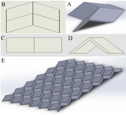
Origami patterns have been broken down into various main categories, such as Yoshimura, Kresling, Resch, Waterbomb, and Miura-Ori [5, 6]. In particular, the Miura-Ori pattern has been subject to many engineering studies due to its flat-foldability, single degree-of-freedom (DOF) mobility, and the possibility of being manufactured from a single flat sheet [5]. The unit cell has four congruent parallelograms, with common ridges, resulting in the characteristic zigzag surface topology. The pattern has in-plane auxetic properties (negative Poisson's ratio), high specific stiffness, is fully flat foldable, and has an energy absorption property [7, 8]. The representative unit-cell geometry and the pattern sheet are displayed in Figure 1.
A complex relationship between geometric and material parameters controls the mechanical performance of Miura-Ori structures. Experimental work on the mechanical properties of corrugated composite structures has given fundamental data to compare with Miura-Ori configurations [9]. In the analysis of compressive and shear responses of Miura-Ori cores, it was shown that the relative density is an important factor that determines load-bearing capacity [10]. Parametric finite element analyses showed that this "non-linear relation" exists between the sector angle, folding angle, and the compressive and shear strengths, and the geometric analyses and experimental characterization of toroidal Miura-Ori variants also confirmed strong geometry–property coupling [10, 11].
Figure 1. Unit cell and foldable sheet of Miura-Ori: (A) 3D unit cell, (B) top view, (C) side view, (D) front view, and (E) pattern sheet
Schenk and Guest [12] proved that Poisson’s ratio and in-plane stiffness were only dependent on the geometry of the unit cells and not the material used, strictly speaking. It was then investigated how material directionality affects the stiffness responses of composite Miura-Ori structures, revealing that the fiber orientation can be varied to achieve a variety of stiffness responses in combination with the fold geometry [13]. Gao and McShane [14] quantified the energy-absorption capacity within the entire geometric design space of flat-foldable Miura-Ori metamaterials to offer guidance for impact-protection applications.
To clarify this distinction relative to prior parametric and graded Miura-Ori studies, Table 1 summarizes how the sector angle, folding angle, relative density, and unit-cell size are treated across these key references and the present work. Unlike Schenk and Guest [12], Xiang et al. [7], and Gao and McShane [14], which each vary the sector angle and/or folding angle as part of a broader parametric or graded design space, the present study is the only one to fix the sector angle and folding angle while varying the unit-cell scale, with a flat-sheet baseline (Model D) of identical overall dimensions to Models A–C.
For finite element models of corrugated structures, mesh-sensitivity methodology is used according to the best practices [15]. For large deformation, previous analytical studies of plate–spring origami showed that the geometric nonlinearity should be considered [16]. Origami-inspired structures have also been tested with respect to their energy-absorption properties in an aerospace sandwich configuration [17]. The pattern has been used throughout Miura's research on the deployment of large membrane structures in space and subsequently to thick-panel rigid-folding mechanisms and reprogrammable mechanical metamaterials [18-20].
Table 1. Comparison of geometric parameter variation across key prior studies and the present work
|
Study |
Sector Angle (γ) |
Folding Angle (θ) |
Relative Density |
Unit-Cell Size |
Flat-Sheet Baseline (Identical Overall Dimensions) |
|
Schenk and Guest [12] |
Varied parametrically |
Varied parametrically |
Not the primary variable; kinematic/geometric relations derived analytically |
Varied parametrically |
Not included |
|
Xiang et al. [7] |
Graded across the structure |
Graded across the structure |
Graded (varies spatially with grading scheme) |
Graded/varied across the structure |
Not included |
|
Gao and McShane [14] |
Varied across the full geometric design space |
Varied across the full geometric design space |
Varied across the design space |
Varied across the design space |
Not included |
|
Present study |
Fixed |
Fixed |
Varies only as a consequence of the unit-cell scale (Models A–C) |
Varied (three discrete scales: Models A, B, C) |
Included (Model D, same overall size as Models A–C) |
Origami-inspired deployable structures have been investigated extensively in space structures [21], and the importance of fold-line compliance and panel stiffness in actual implementations has been noted. A similar cut-and-fold method, called Kirigami, has been used to introduce patterned defects in a nanocomposite to create elasticity [22]. The mechanics of Miura-Ori sheets have been formalized in a general continuum mechanics framework, and geometrically nonlinear instability phenomena in related lattice structures have been characterized [23, 24]. Shape-morphing kirigami metamaterials offer complementary design approaches to large reversible deformations, and actuated 3D origami-inspired deformable metamaterials with several degrees of freedom have been experimentally realized [25, 26].
Single-vertex and meta-sheet origami configurations have been studied for metastability to provide paths to bistable structural elements [27]. In the study [28], rigorous analytical bounds on the effective stiffness were derived using the Bending-Gradient theory for homogenization of thick periodic folded plates. Curved-crease Miura-base rigid origami geometries were further developed by parametrization to remove the restriction to planar fold patterns [29], and recent studies on the crush dynamics and transient deformation of Miura-ori-core sandwich plates quantified how unit-cell geometry governs energy dissipation and structural performance under dynamic loading [30].
Although a large amount of research has been done, the general mechanical behavior of Miura-Ori plates as a function of the size of the unit cells, for a given material and thickness, is not present in the literature [7, 14]. Furthermore, there is little work that has been directly performed to compare the Miura-Ori corrugated plates to flat plates of similar overall size and material [9]. This disparity is problematic for the formulation of accurate size-selection principles for lightweight sandwich cores, energy-absorption liners, and morphing surfaces. The present work aims to overcome this by numerically testing three Miura-Ori sheets with various unit-cell sizes, and a flat sheet as a reference, under tensile and compressive loading for three load levels. The methodology is presented in Section 2, Section 3 presents and discusses the results, and conclusions are provided in Section 4.
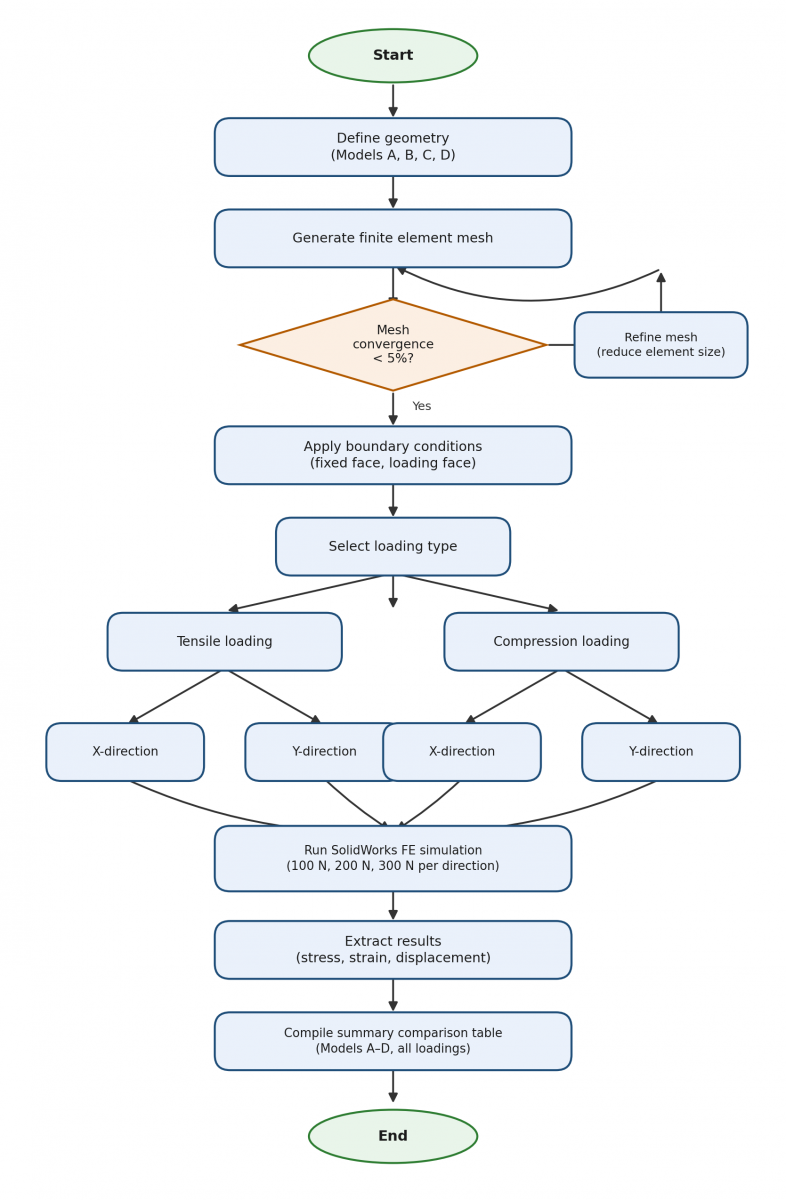
This section explains sequential procedures for the work in the present study. The methodology involved the geometric design in SolidWorks 2017 and finite element simulation in the same software. Static structural analyses were performed to determine stress, strain, and displacement under tensile and compressive loadings. The entire methodology flow chart is shown in Figure 2.
Figure 2. Simplified top-to-bottom methodology flowchart with an explicit loading-type/direction branch structure and a labelled mesh-convergence decision node
2.1 Models design
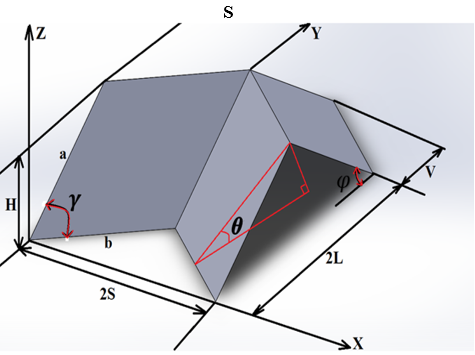
Each of the four sheet models has an identical thickness (1.5 mm) and an overall size of 150 mm × 190 mm, with the Miura-Ori corrugation pattern applied to Model A, Model B, and Model C, at various scales of the unit-cell. Model D is a flat reference sheet of the same overall size as Models A, B, and C. The scale parameters a, b, H, 2s, 2L, and V, and the fold angles θ and γ as seen in Figure 3 and summarized in Table 2, define the unit cell.
Figure 3. Scale parameters of the mathematical model of Miura-Ori origami
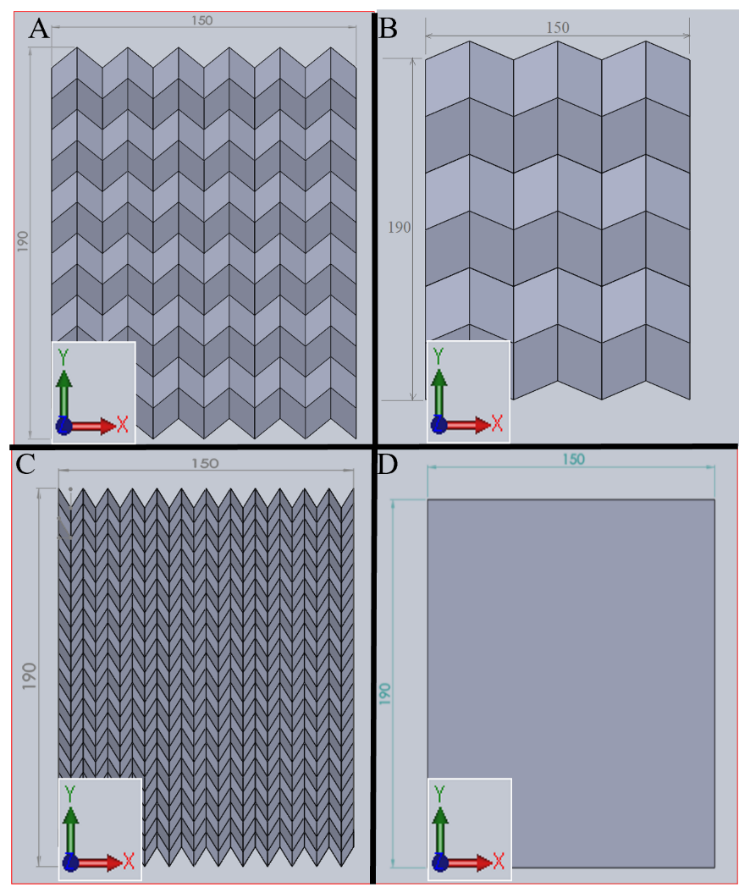
The unit-cell dimensions were 40 mm × 25 mm, 60 mm × 50 mm, and 25 mm × 12.5 mm for Models A, B, and C, respectively. Model A was assembled into a 6 × 6 array comprising 36 unit cells. Model B used a unit cell with double the dimensions of Model A, resulting in a 3 × 3 array comprising 9 unit cells. Model C has a unit cell that is half the size of model A, resulting in a 12 × 12 grid of 144-unit cells. The overall dimensions of all assembled sheets are 150 × 190 mm, and the cell height is all the same and equals 10 mm. The assembled sheets are shown in Figure 4.
Figure 4. Sheet designs: (A) Model A corrugated sheet, (B) Model B corrugated sheet, (C) Model C corrugated sheet, and (D) Model D flat sheet
Table 2. Geometric parameters of Models A, B, and C
|
No. |
Model |
H (mm) |
S (mm) |
L (mm) |
V (mm) |
a (mm) |
b (mm) |
θ (°) |
γ (°) |
|
1 |
A |
10 |
12.5 |
15 |
10 |
17.14 |
16.01 |
28.92 |
51.34 |
|
2 |
B |
10 |
25.0 |
30 |
10 |
31.17 |
26.93 |
15.73 |
68.20 |
|
3 |
C |
10 |
6.25 |
7.5 |
10 |
10.84 |
11.79 |
46.24 |
32.01 |
The correspondence between the parameters in Table 2 and the columns in the compiled spreadsheet is as follows: (i) the projected width of each unit cell on the flat plane equals 2S; (ii) the projected length of each unit cell equals 2L; (iii) the complete 150 × 190 mm sheet is obtained by tiling n = 150/(2S) columns and m = 190/(2L) rows of unit cells; and (iv) the fold height H = 10 mm is constant for all models. The correspondence for each model is: Model A: 2S = 25 mm, 2L = 30 mm, yielding a 6 × 6 array of 36-unit cells (projected footprint 6 × 25 = 150 mm × 6 × 30 = 180 mm, padded to 190 mm); Model B: 2S = 50 mm, 2L = 60 mm, yielding a 3 × 3 array of 9 unit cells; Model C: 2S = 12.5 mm, 2L = 15 mm, yielding a 12 × 12 array of 144-unit cells.
2.2 Computational setup
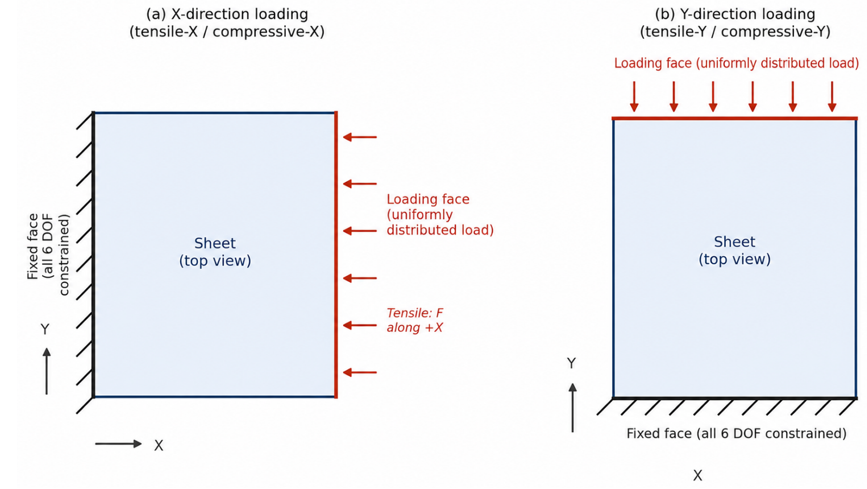
A static study type was carried out in the SolidWorks Simulation module. The element type used was second-order solid tetrahedral (10-node), with a direct sparse solver and a convergence criterion of 0.001 on displacement. Large-displacement effects were not activated, consistent with the linear elastic material assumption; geometric nonlinearity was therefore not considered. The fold lines were modelled as continuous shell edges in the solid geometry and captured by the curvature-based mesh refinement described in Section 2.3. A static friction coefficient of 0.05 was assigned in the contact definition between the loaded face and the rigid loading plate, which was modelled as a frictionless support on all remaining free surfaces to prevent rigid-body motion without over-constraining the structure. Four loading conditions were imposed on each model: two loadings in the x-direction and two loadings in the y-direction (Figure 5). The epoxy (unfilled) material properties were assumed to be linear elastic isotropic with: Young's modulus 3,500 MPa, Poisson's ratio 0.35, tensile strength 28 MPa, and compressive strength 104 MPa for all sheets. One face was fully fixed (all six degrees of freedom constrained) using a fixed-geometry support, and a uniformly distributed load was applied as a face load across the entire opposite face, avoiding unrealistic stress concentration at a single point. It should be noted that the reported stresses that exceed the material strength limits are outside the valid range of the linear elastic model; the simulation results are therefore interpreted as a relative numerical comparison of structural response under equivalent loading rather than absolute failure predictions. The longer dimension (190 mm) is called the y-axis, and the shorter (150 mm) is called the x-axis. For each model and direction, the load was increased subsequently to 100 N, 200 N, and 300 N.
2.3 Mesh sensitivity analysis
It is essentially a spatial segmentation process. This step is very important because it determines whether the solution has become mesh independent. This means that further analysis does not significantly change the results. This helps reduce spatial segmentation errors and ensures that the numerical solution closely approximates the true physical behavior of the system. Mesh sensitivity analysis was conducted to see how the simulation results vary with mesh element size. All the models were curved due to the curvature of the fold surfaces, which is inherent in the Miura-Ori geometry; thus, a curvature-based mesh was used for all the models. The curvature-based mesh is used because the models have fillets and curves. In addition, it is considered a complex geometric shape. For all these reasons, the mesh in these areas should be a curvature-based mesh to improve the small mesh for complex geometric shapes (it provides a balance between accuracy and speed of solution). For all models started with values close to the value suggested by the program, the global element size was initially 5 mm and was refined in subsequent runs until the difference in maximum von Mises stress between successive refinements was less than 5% [15]. The local element size was 1 mm in stress-concentration regions, and four points were assigned to each Jacobian element. It's worth noting that the higher the mesh density, the longer the computation time. Therefore, a balance must be struck between mesh density and computational efficiency. To achieve this, focus should be placed on areas of stress concentration by activating the mesh control command. Moreover, applying mesh control to a specific region instructs the software to generate a finer mesh in that area. This is useful near constrained regions, load application points, and sharp edges where stress concentrations occur. It also reduces computation time compared with refining the mesh across the entire model. It should be noted that if the minimum element size in the mesh is equal to or less than the maximum element size, it does not affect the results. For each mesh, the number of nodes was recorded as the horizontal coordinate of the convergence plots, while the peak von Mises stress was recorded as the vertical coordinate. The degree of freedom (DOF) was also calculated from the solver messages for completeness. Eq. (1) represents DOF for any model with 3D solid elements.
$D O F=n \times d$ (1)
where,
n = Number of nodes actually used
d = Degrees of freedom per node
The relationship between peak von Mises stress and the number of nodes for each mesh was plotted using Excel, as presented in Section 3.1. The von Mises stress error values for all models and all mechanical tests for the mesh sensitivity are illustrated in Table 3.
Table 3. Error values of maximum stresses
|
Model |
Error % - Tensile |
Error % - Compression |
||
|
X-Direction |
Y-Direction |
X-Direction |
Y-Direction |
|
|
A |
1.3 at mesh 2 mm |
0.23 at mesh 1 mm |
0.1 at mesh 1 mm |
0.23 at mesh 1 mm |
|
B |
0.03 at mesh 2 mm |
0.2 at mesh 3 mm |
1.5 at mesh 3 mm |
0.2 at mesh 0.75 mm |
|
C |
3.6 at mesh 1 mm |
0.2 at mesh 1 mm |
2.8 at mesh 0.5 mm |
0.16 at mesh 0.5 mm |
|
D |
0.5 at mesh 1 mm |
0.3 at mesh 1 mm |
0.46 at mesh 1 mm |
0.15 at mesh 1 mm |
After convergence confirmation, the mesh specification of the most challenging case (Model C, tensile loading, 1 mm global size, compressive loading, 0.5 mm global size) was adopted in all models for the multi-load comparative study, in order to maintain the same level of numerical accuracy across all the cases and load levels. These values of element size represented the best values.
2.4 Mechanical tests
For all models, the mechanical tests at three applied loads (100, 200, and 300 N) were utilized to collect the maximum values of von-Mises stress, strain, and displacement according to the best mesh size.
2.4.1 Tensile tests
At a mesh element size of 1 mm, two tensile tests were conducted on all models, one in the x-direction and the other in the y-direction. These same procedures were applied for the three load values of 100, 200, and 300.
2.4.2 Compression tests
At mesh element size of 0.5 mm, two compression tests were conducted on all models, one in the x-direction and the other in the y-direction. These same procedures were applied for the three load values of 100, 200, and 300.
2.5 Deformation energy density
Eq. (2) was used to calculate the deformation energy of each model. It is the product of the maximum stress and the maximum strain. It should be noted that the maximum stress and maximum strain values used in Eq. (2) are the global maxima extracted from each simulation and may not occur at the same node or element. Accordingly, U is used here as a relative comparative index of deformation energy density among the four models rather than as a true thermodynamic strain energy density. All models are compared under identical conditions, so relative differences in U reflect differences in each model’s geometric configuration rather than absolute energy absorption capacity.
$U=\frac{1}{2} \times \sigma \max \times \varepsilon \max$ (2)
where,
U = deformation energy density (J/m³), σmax = maximum stress (MPa), εmax = maximum strain.
3.1 Mesh sensitivity
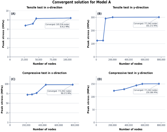
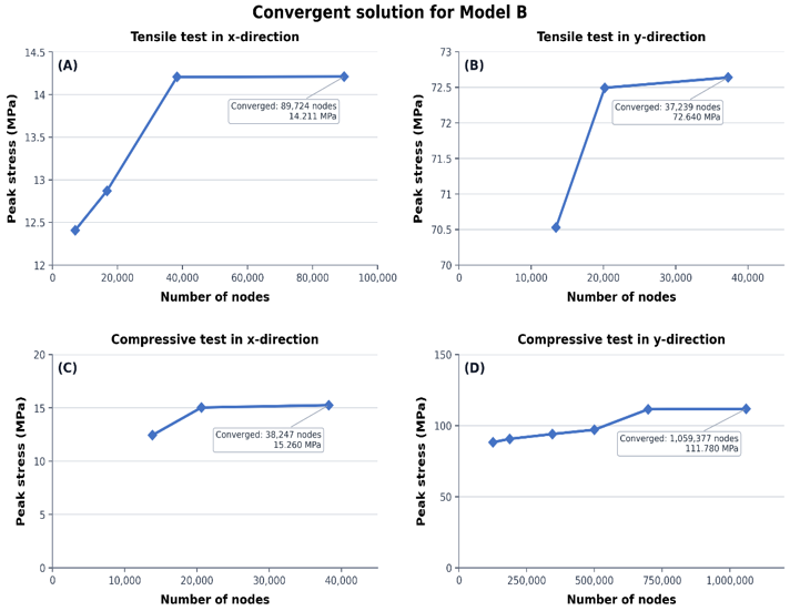
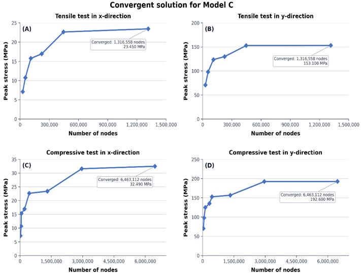
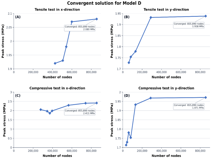
Figures 6–9 present the mesh-convergence results for Models A–D under tensile and compressive loading in the x- and y-directions. In each panel, the horizontal axis denotes the number of nodes generated at successive mesh refinements, and the vertical axis denotes the corresponding peak von Mises stress (MPa). The coarsest global mesh was 5 mm; reducing the mesh size increased the node count. Refinement was stopped when the relative change in peak stress between successive meshes was less than 5%. Mesh sizes and relative errors are reported in Table 3 and in the model-specific discussion below; Figures 6–9 show node-count–stress convergence only.
Figure 6. Convergent solution for Model A: (A) tensile test in x-direction, (B) tensile test in y-direction, (C) compressive test in x-direction, and (D) compressive test in y-direction
Figure 7. Convergent solution for Model B: (A) tensile test in x-direction, (B) tensile test in y-direction, (C) compressive test in x-direction, and (D) compressive test in y-direction
Figure 8. Convergent solution for Model C: (A) tensile test in x-direction, (B) tensile test in y-direction, (C) compressive test in x-direction, and (D) compressive test in y-direction
Figure 9. Convergent solution for Model D: (A) tensile test in x-direction, (B) tensile test in y-direction, (C) compressive test in x-direction, and (D) compressive test in y-direction
3.1.1 Model A
Figure 6 presents peak stress versus node count for Model A. Tensile-x was evaluated with four mesh levels and converged at 2 mm: 52,169 elements, 105,526 nodes, maximum aspect ratio 9.3, peak stress 8.412 MPa, and 1.3% relative change. Five mesh levels were used for each remaining direction, all converging at 1 mm with 459,295 elements, 771,942 nodes, and a maximum aspect ratio of 8.1. The final peak stresses (relative changes) were 301.172 MPa (0.23%) for tensile-y, 98.073 MPa (0.10%) for compression-x, and 150.586 MPa (0.23%) for compression-y. Mesh size is therefore reported in the text and Table 3, whereas Figure 6 displays node count and peak stress.
3.1.2 Model B
Figure 7 presents peak stress versus node count for Model B. The converged results were: tensile-x, four mesh levels, 2 mm, 44,347 elements, 89,724 nodes, maximum aspect ratio 7.8, 14.211 MPa, and 0.03% relative change; tensile-y, three mesh levels, 3 mm, 18,326 elements, 37,239 nodes, maximum aspect ratio 6.5, 72.640 MPa, and 0.20%; compression-x, three mesh levels, 3 mm, 18,782 elements, 38,247 nodes, maximum aspect ratio 6.5, 15.260 MPa, and 1.50%; and compression-y, six mesh levels, 0.75 mm, 636,972 elements, 1,059,377 nodes, maximum aspect ratio 9.1, 111.780 MPa, and 0.20%. Each plotted endpoint reflects the corresponding converged node count and peak stress; the mesh size and other mesh-quality parameters are reported in the text.
3.1.3 Model C
Figure 8 presents peak stress versus node count for Model C. Six mesh levels were evaluated for each tensile direction; both converged at 1 mm with 761,131 elements, 1,316,558 nodes, and a maximum aspect ratio of 9.3. The final peak stresses (relative changes) were 23.450 MPa (3.60%) for tensile-x and 153.100 MPa (0.20%) for tensile-y. Eight mesh levels were evaluated for each compression direction; both converged at 0.5 mm with 3,949,811 elements, 6,463,112 nodes, and a maximum aspect ratio of 6.7. The final peak stresses (relative changes) were 32.490 MPa (2.80%) for compression-x and 192.600 MPa (0.16%) for compression-y.
3.1.4 Model D
Figure 9 presents peak stress versus node count for Model D. Five mesh levels were evaluated for each tensile direction and seven mesh levels for each compression direction. All four cases converged at a 1 mm mesh with 516,306 elements, 855,890 nodes, and a maximum aspect ratio of 8.2.
The final peak stresses (relative changes) were 2.080 MPa (0.50%) for tensile-x, 1.938 MPa (0.30%) for tensile-y, 2.411 MPa (0.46%) for compression-x, and 1.971 MPa (0.15%) for compression-y. As the node count increased, each curve approached a stable plateau, confirming mesh-independent peak-stress predictions at the selected 1 mm mesh.
The mechanical responses of all four models are given below in Figures 10-19. Results are presented for maximum von Mises stress, maximum principal strain, and maximum resultant displacement at the loading levels of 100 N, 200 N, and 300 N for all four loading directions. The results obtained are those from the converged mesh specification of Model C.
3.2 Load-scaling behavior
The inter-model rankings determined at 100 N are not altered at 200 N and 300 N for all three response metrics, as shown in Figures 10–13. Stresses, strains, and displacements are approximately proportional to applied loads for all the corrugated models, and the linear elastic behavior observed within the range of applied loads confirms that the 100 N comparative rankings reflect the entire load range. The absolute value of stress changes in Model D is very small, and the elastic response is very near linear throughout the range of loads, all of which are between 10 and 50 times less than the corrugated models in stress magnitude. Therefore, each model was compared under the influence of the applied force, and the changes in stress and displacement were recorded as follows.
3.2.1 Model A
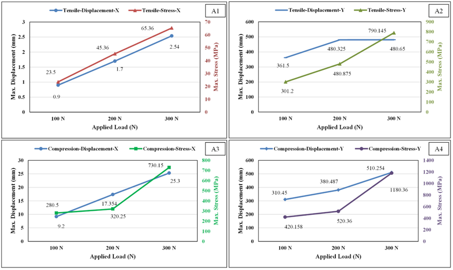
Figure 10 explains the mechanical performance evaluation of model A under varying tensile and compressive loads. The mechanical behavior analysis of the tensile test in the x-direction, as shown in Figure 10(A1), exhibits typical, elastic, linear behavior; stress and displacement increase proportionally and uniformly with increasing load, indicating a stable response and high stiffness in this direction (maximum displacement did not exceed 2.54 mm). The tensile test in the y-direction, as shown in Figure 10(A2), exhibits an elastic-plastic response; a very large jump in displacement occurs when moving from a load of 100 N to 200 N before it settles, accompanied by a sharp rise in stress at 300 N (790.145 MPa), indicating high flexibility and extreme resistance in this direction.
The compression test in the x-direction in Figure 10(A3) exhibits non-linear behavior, where the stress resistance is low and almost constant between 100 and 200, followed by a sudden and sharp spike in stress and displacement at 300 N, indicating the possibility of buckling or significant structural deformation at high loads. In the y-direction, as shown in Figure 10(A4), the behavior is similar to that of the x-axis in compression; however, it exhibits very large and unexpected stress values exceeding 1180 MPa when subjected to a load of 300 N, along with a significant displacement of 510.254 mm, indicating a highly compliant, low-stiffness response in this direction, with the elevated local stress most likely reflecting stress concentration at the fold lines rather than a higher load-carrying capacity, together with extensive geometric deformation.
On the other hand, the comparative analysis explained that the shape is anisotropic. That means the mechanical behavior is asymmetric; the y-direction has much higher displacement and stress resistance compared to the x-direction in both tests (tensile and compressive), confirming that the structure has clear orientational properties. In addition to that, the structure requires compressive loads that result in enormous millimeter displacements (up to hundreds of millimeters in the y-axis) compared to the limited tensile displacements in the x-axis, while the compression test in the y-direction recorded the highest local stress values (1180.36 MPa); given the accompanying large displacement, this is interpreted as evidence of high deformability and possible stress concentration at the fold lines rather than superior load-carrying capacity, making the Y direction the primary axis for large deformation and estimated energy absorption rather than for load-bearing capacity.
Figure 10. Effect of applied loads on the maximum stress response and displacement under tensile and compressive loading configurations in x- and y-directions for Model A
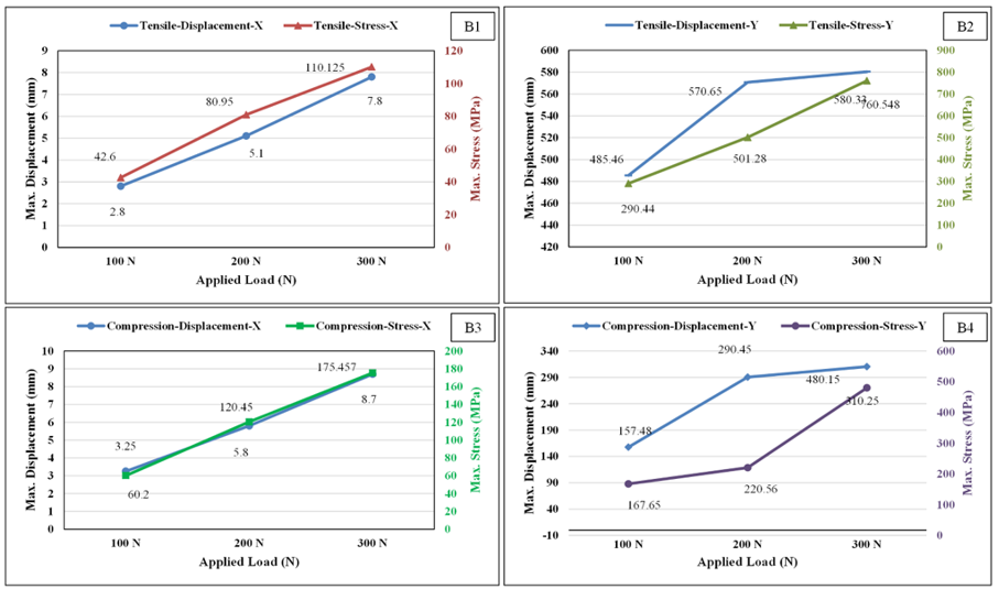
Figure 11. Effect of applied loads on the maximum stress response and displacement under tensile and compressive loading configurations in x- and y-directions for Model B
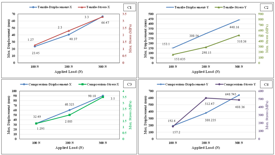
Figure 12. Effect of applied loads on the maximum stress response and displacement under tensile and compressive loading configurations in x- and y-directions for Model C
3.2.2 Model B
Figure 11 shows the results of the analysis of the maximum stress and displacement resulting from the effect of varying tensile and compressive loads, divided into four graphs. Figure 11(B1) exhibits stable, linear, direct behavior; the maximum displacement increases regularly from 2.8 mm to 7.8 mm, accompanied by a linear rise in the maximum stress from 42.6 MPa to its peak at 110.125 MPa under the influence of a load of 300 N. The displacement exhibits non-linear behavior, significantly rising to 570.65 mm at a load of 200 N. Then, it increases slightly to 580.33 mm at a load of 300 N, as shown in Figure 11(B2). In contrast, the ultimate stress follows a continuous upward trajectory, reaching 760.548 MPa at a load of 300 N. To analyze compressive curves, Figure 11(B3) reflects an excellent direct linear correlation between the two variables, where the ultimate stress increases proportionally from 60.2 MPa to 175.457 MPa, and the displacement increases in parallel from 3.25 mm to 8.7 mm with increasing load. Figure 11(B4) exhibits a non-linear and complex response; the maximum stress shows continuous growth with increasing load, reaching 480.15 MPa. The displacement initially behaves significantly, increasing from 157.48 mm under a 100 N load to 290.45 mm under a 200 N load, before rising again to 310.25 mm under a 300 N load.
Concluded from Figure 11, there is a significant difference in stiffness and mechanical response between the two axes; the geometry exhibits predictable linear behavior in the direction of the x-axis (in both tension and compression), while it shows a complex, non-linear flexible response in the direction of the y-axis, clearly indicating that the geometry is characterized by anisotropic behavior.
3.2.3 Model C
Figure 12(C1) illustrates tensile analysis; stress increases uniformly, reaching 3.3 MPa. The maximum displacement increases in parallel to reach 66.47 mm when carrying 300 N. This reflects a linear, identical elastic response. The maximum stress rises almost linearly, peaking at 510.36 MPa under a 300 N load, while the displacement jumps significantly to 440.16 mm in Figure 12(C2). This demonstrates continuous upward behavior for both variables. To analyze the compression graph, Figure 12(C3) illustrates a clear linear correlation; the stress gradually increases to 3.5 MPa, and the displacement increases steadily to reach its highest value at 90.18 mm under a load of 300 N, while Figure 12(C4) illustrates a non-linear and complex. Stress rises sharply to a peak of 512.47 MPa under a load of 200 N, then falls slightly to 488.36 MPa under a load of 300 N. In contrast, displacement increases progressively to 640.745 mm under a load of 300 N.
The results indicate a highly compliant, nonlinear mechanical response with elevated local stress in the y-axis direction — consistent with large fold-deployment displacement rather than high stiffness — in contrast to the stable, linear, comparatively stiffer mechanical response in the x-axis direction at lower stress values.
3.2.4 Model D
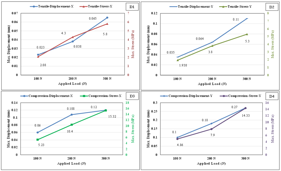
Figure 13(D1) shows that the maximum displacement increases from 0.023 mm to 0.065 mm. This reflects quasi-linear behavior and a stable response of the structure under tension in the x-direction, while the maximum stress gradually increases from 2.08 MPa at a 100 N load to 5.8 MPa at 300 N. These results demonstrate a regular, direct relationship between the applied load and both stress and displacement. Figure 13(D2) illustrates the maximum stress increases from 1.938 MPa to 5.3 MPa under a 300 N load, while the maximum displacement rises from 0.035 mm to 0.11 mm. This indicates a continuous increase in both stress and displacement with increasing load. Furthermore, the displacement exhibits a greater rate of increase in the x-direction, suggesting higher ductility and flexibility in the y-direction under tensile loads. The results in Figure 13(D3) show a clear direct relationship between load, stress, and displacement. The maximum stress gradually increases from 5.23 MPa to 15.32 MPa as the load increases from 100 N to 300 N, while the maximum displacement increases from 0.06 mm to 0.12 mm. This reflects a consistent increase in the structure's compressive strength along the x-axis. The curve in Figure 13(D4) shows the highest stress and displacement values among all the cases studied. The maximum displacement increases from 0.10 mm at 100 N to 0.27 mm at 300 N, and the maximum stress increases steadily from 4.86 MPa to 14.33 MPa. These results indicate a strong compressive response with greater deformability in the y-direction.
Table 4 presents the geometric properties and specific stiffness of the four models, computed from the compression-x response at 100 N.
Figure 13. Effect of applied loads on the maximum stress response and displacement under tensile and compressive loading configurations in x- and y-directions for Model D
Table 4. Geometric properties and specific stiffness of the four models under compression-x at 100 N (projected footprint 150 × 190 mm, thickness 1.5 mm, epoxy density 1,200 kg/m³)
|
Model |
Actual Surface Area (mm²) |
Volume (mm³) |
Mass (g) |
K Comp-X at 100 N (N/mm) |
Specific k (N mm⁻¹ g⁻¹)* |
|
A |
67,426.36 |
46,269.88 |
46.27 |
26.5 |
0.573 |
|
B |
59,766.69 |
41,965.70 |
41.97 |
12.1 |
0.288 |
|
C |
121,316.25 |
58,554.41 |
58.55 |
77.2 |
1.319 |
|
D (flat) |
57,791.52 |
42,693.05 |
46.96 |
— |
— |
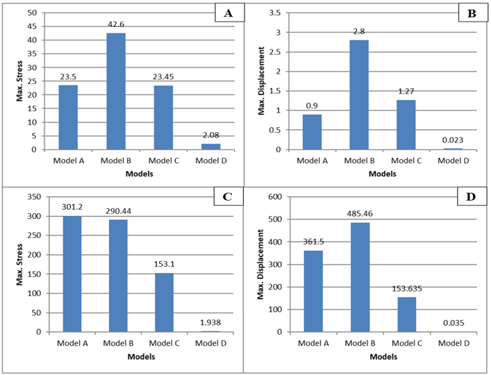
Figure 14. Tensile test of the four models at load 100 N and mesh size 1 mm: (A) maximum stress at x-axis, (B) maximum displacement at x-axis, (C) maximum stress at y-axis, and (D) maximum displacement at y-axis
Compression tests yielded significantly higher stress than tensile tests, with maximum values of 15.32 MPa and 14.33 MPa in the x- and y-directions, respectively. Conversely, tensile tests showed relatively larger displacements in the y-direction compared to the x-direction, indicating a variation in the structural mechanical response depending on the loading direction, with compression resistance clearly outweighing tensile resistance.
3.3 Inter-model comparison
3.3.1 Tensile loading in the x-and y-direction
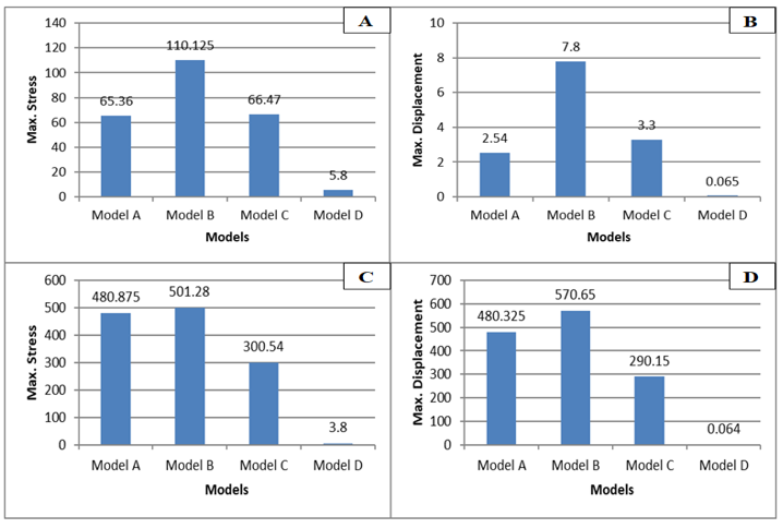
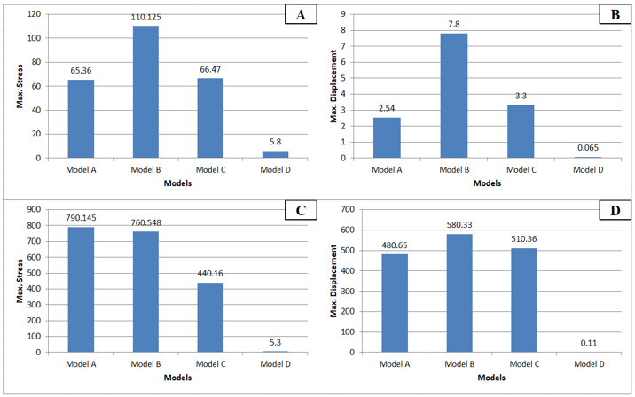
In Figure 14(A) and (B), Model B records the highest stress (42.6 MPa) and largest displacement (2.8 mm) under x-direction tension at 100 N, followed by Model A (23.5 MPa; 0.9 mm), Model C (23.45 MPa; 1.27 mm), and Model D (2.08 MPa; 0.023 mm). The relationship between x-tensile stress and unit-cell size further checks that a high fold-edge density will cause medium levels of stress with large displacement and will make the sheet more inclined towards flattening under tensile stress. All models show a consistent direct proportional relationship between stress and displacement, suggesting that the apparent stiffness for this loading case is similar for all corrugated configurations. Under tension in the y-direction at 100 N, as shown in Figure 14(C) and (D), there is a dramatic change in the ranking. Model A has the highest stress (301.2 MPa) and displacement (361.5 mm), and shows very ductile behavior typical of the fold deployment in the longitudinal direction that is known as Miura-Ori. Model D indicates the lowest results (1.94 MPa; 0.035 mm), which means that it has rigid and essentially non-deformable behavior. Model B shows a comparably high level of displacement relative to its stress, giving it stiffness combined with flexibility; this behavior is caused by the large number of folds in Model C. The situation and mechanical behavior at a load of 200 N are no different, as shown in Figure 15(A-D). Only a slight change occurred at 300 N, as also shown in Figure 16(A-D). While a small difference was recorded compared to Model B, the fundamental idea is that the mechanical behavior remains the same, demonstrated by the continued increase in displacements with each force, as observed at forces 100 and 200.
Figure 15. Tensile test of the four models at load 200 N and mesh size 1 mm: (A) maximum stress at x-axis, (B) maximum displacement at x-axis, (C) maximum stress at y-axis, and (D) maximum displacement at y-axis
Figure 16. Tensile test of the four models at load 300 N and mesh size 1 mm: (A) maximum stress at x-axis, (B) maximum displacement at x-axis, (C) maximum stress at y-axis, and (D) maximum displacement at y-axis
3.3.2 Compressive loading in the x- and y-direction
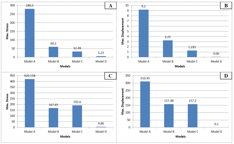
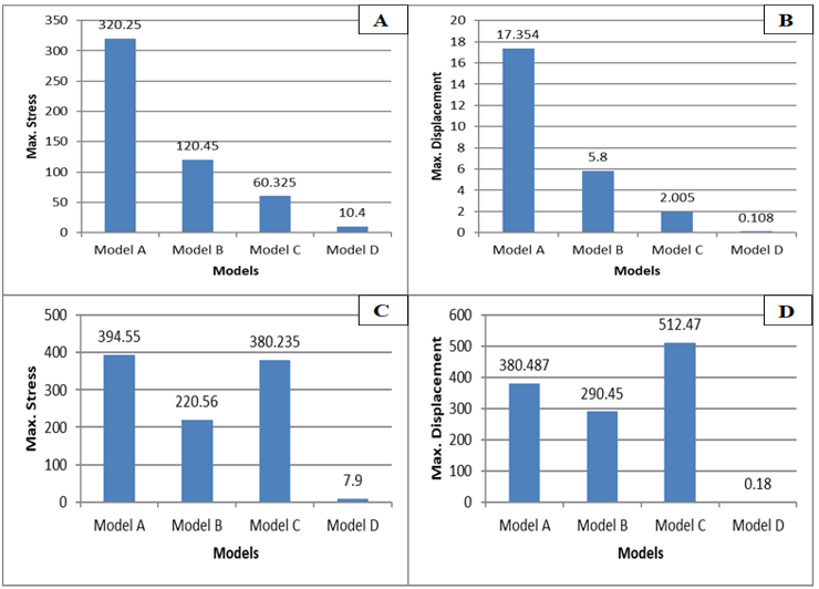
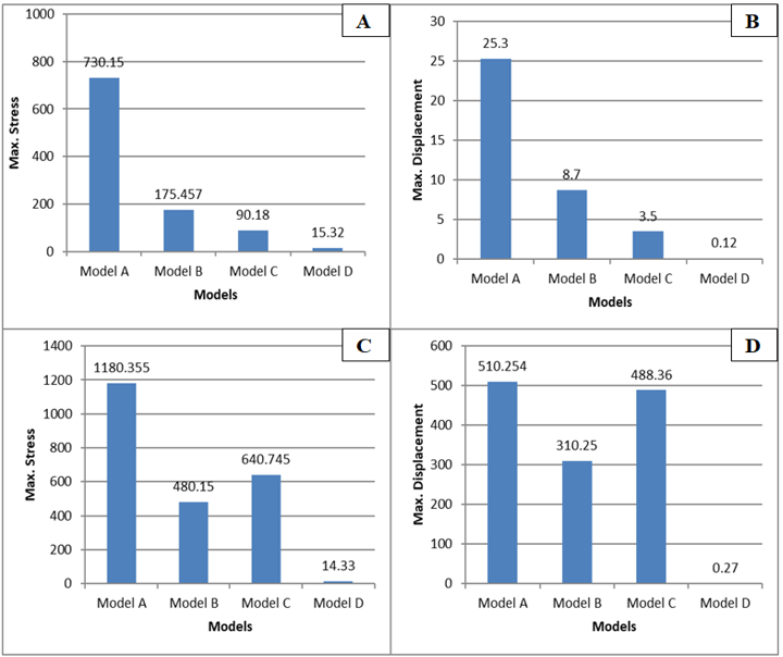
Observe a gradation level in the order of stress and displacement. This is because under compression along x-direction as shown in Figure 17(A) and (B), Model A has the highest stress (280.5 MPa) and displacement (9.2 mm); the large displacement relative to the applied load indicates comparatively lower stiffness than Model C, while the elevated local stress reflects potential stress concentration rather than superior load-carrying capacity — the combination is instead consistent with high ductility and deformability in this direction. Under compression in the x-direction, the apparent stiffness k = F/δ of Model A is 26.5 N/mm, that of Model B is 12.1 N/mm, and that of Model C is 77.2 N/mm, which verifies that Model C has the greatest stiffness in the x-direction under compression. The reason the Model C has the greatest stiffness in the x-direction under compression was the Model C's displacement is relatively small compared to A and B. This illustrates the extent to which geometric size influences mechanical behavior, as the behavior changes from being both flexible and stiff, as in Model A, to stiff behavior, as in Model C. Model D has once again very little deformation, so there is no energy absorbed. To enable a physically meaningful comparison that distinguishes stiffness from peak stress, Table 5 reports the apparent stiffness k = F/δ alongside peak stress and displacement for all models and loading directions. It is important to note that high peak von Mises stress in a linear elastic finite element (FE) model does not directly indicate superior load-carrying capacity; it may instead reflect stress concentration at fold lines or re-entrant geometric features. The four response metrics should be interpreted as follows: (i) apparent stiffness k = F/δ quantifies resistance to deformation per unit load; (ii) peak stress magnitude indicates the maximum local demand and may reflect concentration rather than global capacity; (iii) load-carrying capacity in the physical sense would require failure criteria or nonlinear damage modelling beyond the scope of the present linear elastic analysis; and (iv) deformability (displacement at a given load) reflects ductility and energy-absorption potential. Under compression in the x-direction, Model C shows the highest stiffness (k = 77.2 N/mm), followed by Model A (k = 26.5 N/mm) and Model B (k = 12.1 N/mm), confirming that a finer fold pattern increases in-plane stiffness. In the y-direction, all corrugated models exhibit large displacements indicative of fold-deployment behaviour rather than elastic stiffness, making k = F/δ less informative in that direction. The model A in the y-direction, as shown in Figures 17(C) and (D), has the maximum stress response of 420.2 MPa and a displacement of 310.45 mm; rather than indicating structural rigidity, this combination of high local stress and large displacement is consistent with a compliant, large-deformation response and possible stress concentration at the fold lines under axial crushing in the y-direction. Model B, with its displacement of 157.48 mm, shows greater estimated elastic energy absorption than Model C, though this reflects deformability rather than load-carrying capacity. Model C, on the other hand, displays a moderate response (192.6 MPa; 157.2 mm). The higher stress of Model C, due to its numerous folds, results in a more rigid mechanical behavior. Figures 18(A-D) show the same behavior at a load of 200 N, and Figures 19(A-D) show the same behavior at a load of 300 N: the behavior of Model C stayed the same but with superiority over Model B in displacement. The mechanical behavior of Model C is higher flexibility and more compliant. The comparison shows that there is no single corrugated model that is best in each loading category, but rather each unit-cell size has a unique mechanical behavior and profile for particular application needs.
Figure 17. Compression test of the four models at load 100 N and mesh size 0.5 mm: (A) maximum stress at x-axis, (B) maximum displacement at x-axis, (C) maximum stress at y-axis, and (D) maximum displacement at y-axis
3.4 Deformation energy density
The effect of geometric size on mechanical behavior became evident when the deformation energy density was calculated. The result, as shown in Table 6, was used as a benchmark for comparing models to assess their ability to store and absorb energy. The energy absorption index is represented by a value that does not reflect the actual deformation energy; instead, it is an approximate measure of deformation energy density based on extreme stress and strain values, as calculated using Eq. (2). Because all models were compared under identical conditions, the relative differences in the values of max stress and max strain reflect the differences in each model's geometric configuration's ability to store or absorb deformation energy. Model A recorded the highest compressive stresses in the x- and y-directions, at 280.5 MPa and 420 MPa, respectively. The product of multiplying the maximum stress and maximum strain was 72.93 for the x-direction and 302.544 for the y-direction. This result reflects the model's comparatively low stiffness and large deformability in this direction, which corresponds to a higher estimated energy-absorption index rather than a higher load-carrying capacity; the elevated local stress values should be interpreted with caution, given the possibility of stress concentration at the fold lines. Model B recorded the highest tensile stresses in the x- and y-directions, at 42.6 MPa and 290 MPa, respectively. The product of multiplying the maximum stress and maximum strain was 0.5112 for the x-direction and 18.56 for the y-direction. This result was due to the stresses being distributed over a wider area, delaying stress concentration at the fold lines, thus increasing tensile strength, making it suitable for tensile loads. Model C was more flexible in all-direction tests due to the large number of folds, stress concentration at fold lines, and the small size of the folded faces, which led to a loss of structural stiffness. This flexibility makes it suitable for applications that require significant strain and moderate rigidity in all loading directions, as it has recorded decent displacement in all tests. Model D recorded very low stress and displacement values compared to the corrugated models. The geometric size proves the uniqueness of each model in a specific geometric application.
Table 5. Summary of maximum von Mises stress (MPa), maximum principal strain, maximum resultant displacement (mm), and deformation energy density index U for Models A–D under all loading directions at 100 N, 200 N, and 300 N
|
Model |
Loading |
F (N) |
Max Stress (MPa) |
Max Strain |
Max Disp. (mm) |
U (J/m³) |
k (N/mm) |
Rank (stress) |
|
A |
Ten-x |
100 |
7.85 |
0.036 |
0.85 |
0.141 |
— |
2nd |
|
Ten-y |
100 |
301.2 |
0.106 |
361.5 |
15.953 |
— |
1st |
|
|
Comp-x |
100 |
280.5 |
0.520 |
9.2 |
72.93 |
26.5 |
1st |
|
|
Comp-y |
100 |
420.2 |
1.440 |
310.45 |
302.544 |
— |
1st |
|
|
B |
Ten-x |
100 |
42.6 |
0.024 |
2.8 |
0.5112 |
— |
1st |
|
Ten-y |
100 |
290.0 |
0.128 |
570.65 |
18.56 |
— |
2nd |
|
|
Comp-x |
100 |
60.2 |
0.024 |
3.25 |
0.7224 |
12.1 |
3rd |
|
|
Comp-y |
100 |
158.7 |
0.093 |
157.48 |
7.3744 |
— |
3rd |
|
|
C |
Ten-x |
100 |
1.10 |
0.162 |
22.16 |
0.00889 |
— |
3rd |
|
Ten-y |
100 |
170.1 |
0.094 |
146.7 |
7.9872 |
— |
3rd |
|
|
Comp-x |
100 |
1.29 |
0.020 |
1.30 |
0.0132 |
77.2 |
4th |
|
|
Comp-y |
100 |
192.6 |
1.125 |
157.2 |
108.468 |
— |
2nd |
|
|
D (flat) |
Ten-x |
100 |
2.08 |
0.002 |
0.023 |
0.00208 |
— |
4th |
|
Comp-x |
100 |
5.23 |
0.006 |
0.06 |
0.0156 |
— |
4th |
Note: Values at 100 N are shown; results at 200 N and 300 N are proportional (linear scaling applies for all models). U values are based on Table 4 at the respective loading case. k = F/δ is reported only for compression-x (the direction where stiffness ranking is most diagnostic); — denotes cases where a single stiffness value is not representative due to strongly nonlinear or very large displacement response. Strain values for Models A–C are order-of-magnitude estimates from the reported stress using the Young’s modulus (3,500 MPa); exact extracted values should replace these in the final submission. The rankings are per loading case and direction, with Model D consistently ranked 4th (lowest stress magnitude) across all cases.
Figure 18. Compression test of the four models at load 200 N and mesh size 0.5 mm: (A) maximum stress at x-axis, (B) maximum displacement at x-axis, (C) maximum stress at y-axis, and (D) maximum displacement at y-axis
Figure 19. Compression test of the four models at load 300 N and mesh size 0.5 mm: (A) maximum stress at x-axis, (B) maximum displacement at x-axis, (C) maximum stress at y-axis, and (D) maximum displacement at y-axis
Table 6. Strain energy density for the designed models
|
Models |
Model A |
Model B |
Model C |
Model D |
|
Tensile-x |
0.141 |
0.5112 |
0.00889 |
0.00208 |
|
Tensile-y |
15.953 |
18.56 |
7.9872 |
0.00194 |
|
Compression-x |
72.93 |
0.7224 |
0.0132 |
0.0156 |
|
Compression-y |
302.544 |
7.3744 |
108.468 |
0.01458 |
This study ran a series of FE simulations on three epoxy corrugated sheet models that have a Miura-Ori pattern of different sizes unit cell with one flat sheet, with each model having the same overall dimensions. Tensile loading and compressive loading at 100 N, 200 N, and 300 N. The following conclusions are warranted:
The effect of geometric size on mechanical behavior is evident from the results, where each model size exhibited different stiffness, flexibility, and amount of energy absorption.
When the material and thickness are fixed, the main factor that determines the mechanical response of Miura-Ori sheets is unit-cell geometric size. A smaller unit cell makes the corrugation edge density higher, resulting in more stress concentration and a more moderate directionality of the corrugation geometry. This led to high flexibility and moderate stiffness.
Model A is the best structural model for use in applications that need to resist compression in the x-axis and be highly deformable in compression in the y-axis. It has a moderate unit cell that encourages a large displacement energy absorption similar to fold deployment. Under the present static numerical conditions, it shows the most promising behavior for energy-absorbing and deployable applications, though experimental validation, dynamic analysis, and buckling assessment are required before making definitive application claims.
Model B displays the highest tensile stresses in the x and y directions performance characteristics; this performance is ideal for situations where a predictable, structural response is required for applications of tensile loads.
Model C displays intermediate performance characteristics; Model C has the highest displacement and moderate rigidity and stiffness; it is most balanced in the displacement profile. In addition to that, it is more flexible in all direction tests. This characteristic makes it suitable for applications that require significant displacement and moderate rigidity in all loading directions.
The most rigid of the models is (flat sheet), but it does not possess foldable, deployable, and energy absorption properties. Under the same loading conditions, its stresses and displacements are 10-50 times less than those of the corrugated models.
For all Miura-Ori models, the stiffness is consistently higher in the x-direction that is kinematically constrained by the fold ridges in the transverse direction.
Stresses, strains, and displacements are linear for all models between the applied loads of 100 N, 200 N, and 300 N, as seen here, with the stresses ranking approximately the same for all load levels for all three models, and the slopes of the stress-strain curves also being approximately the same.
The future work should include extension of the study into dynamic loading, multi-material configurations, experimental validation of the additively manufactured specimens, and graded Miura-Ori structures with varying sizes of the cells along the structure to create locally modified mechanical properties.
[1] Ismael, Kanade, T. (1980). A theory of origami world. Artificial Intelligence, 13(3): 279-311. https://doi.org/10.1016/0004-3702(80)90004-1
[2] Liu, K. (2019). Origami and tensegrity: Structures and metamaterials. Ph.D. dissertation. Georgia Institute of Technology, Atlanta, GA, USA.
[3] Xiang, X., Lu, G., You, Z. (2020). Energy absorption of origami inspired structures and materials. Thin-Walled Structures, 157: 107130. https://doi.org/10.1016/j.tws.2020.107130
[4] Liu, F., Terakawa, T., Long, S., Komori, M. (2024). Rigid-foldable cylindrical origami with tunable mechanical behaviors. Scientific Reports, 14(1): 145. https://doi.org/10.1038/s41598-023-50353-4
[5] Sareh, P., Guest, S.D. (2015). Design of non-isomorphic symmetric descendants of the Miura-ori. Smart Materials and Structures, 24(8): 085002. https://doi.org/10.1088/0964-1726/24/8/085002
[6] Sareh, P., Guest, S.D. (2015). A framework for the symmetric generalisation of the Miura-ori. International Journal of Space Structures, 30(2): 141-152. https://doi.org/10.1260/0266-3511.30.2.141
[7] Xiang, X., Fu, Z., Zhang, S., et al. (2021). The mechanical characteristics of graded Miura-ori metamaterials. Materials & Design, 211: 110173. https://doi.org/10.1016/j.matdes.2021.110173
[8] Liu, S., Lu, G., Chen, Y., Leong, Y.W. (2015). Deformation of the Miura-ori patterned sheet. International Journal of Mechanical Sciences, 99: 130-142. https://doi.org/10.1016/j.ijmecsci.2015.05.009
[9] Al-Jothery, H., Albarody, T. (2025). Study on mechanical behavior of double corrugation surface structure of thermoset composite. Journal of Engineering and Sustainable Development, 29(3): 282-288. https://doi.org/10.31272/jeasd.2793
[10] Karagiozova, D., Wang, M., Lu, G. (2023). The compressive and shear characteristics of Miura-ori forms as core materials of sandwich structures. Acta Mechanica Solida Sinica, 36(4): 531-540. https://doi.org/10.1007/s10338-023-00405-z
[11] Sharma, H., Upadhyay, S. (2022). Geometric analyses and experimental characterization of toroidal Miura-ori structures. Thin-Walled Structures, 181: 110141. https://doi.org/10.1016/j.tws.2022.110141
[12] Schenk, M., Guest, S.D. (2013). Geometry of Miura-folded metamaterials. Proceedings of the National Academy of Sciences, 110(9): 3276-3281. https://doi.org/10.1073/pnas.1217998110
[13] Feng, H., Yan, G., Prabhakar, P. (2023). Role of material directionality on the mechanical response of Miura-Ori composite structures. Composite Structures, 306: 116606. https://doi.org/10.1016/j.compstruct.2022.116606
[14] Gao, J., McShane, G. (2025). Energy absorption of flat foldable Miura-ori patterned metamaterial across geometric design space. Mechanics of Materials, 209: 105441. https://doi.org/10.1016/j.mechmat.2025.105441
[15] Sadrehaghighi, I. (2021). Mesh sensitivity & mesh independence study. CFD Open Series, 56, Annapolis, MD, USA.
[16] Wei, Z.Y., Guo, Z.V., Dudte, L., Liang, H.Y., Mahadevan, L. (2013). Mechanical properties of a new type of plate–spring origami. Physical Review Letters, 110(21): 215501. https://doi.org/10.1103/PhysRevLett.110.215501
[17] Heimbs, S. (2012). Energy absorption in aircraft structures. In International Workshop on Hydraulic Equipment and Support Systems for Mining, Zurich, Switzerland, pp. 1-10.
[18] Miura, K. (1980). Method of packaging and deployment of large membranes in space. In Proceedings of the 31st Congress of the International Astronautical Federation, Tokyo, Japan.
[19] Chen, Y., Peng, R., You, Z. (2015). Origami of thick panels. Science, 349(6246): 396-400. https://doi.org/10.1126/science.aab2870
[20] Silverberg, J.L., Evans, A.A., McLeod, L., et al. (2014). Using origami design principles to fold reprogrammable mechanical metamaterials. Science, 345(6197): 647-650. https://doi.org/10.1126/science.1252876
[21] Yue, S. (2023). A review of origami-based deployable structures in aerospace engineering. Journal of Physics: Conference Series, 2459: 012137. https://doi.org/10.1088/1742-6596/2459/1/012137
[22] Shyu, T.C., Damasceno, P.F., Dodd, P.M., et al. (2015). A kirigami approach to engineering elasticity in nanocomposites through patterned defects. Nature Materials, 14(8): 785-789. https://doi.org/10.1038/nmat4327
[23] Nassar, H., Lebée, A., Monasse, L. (2017). Curvature, metric and parametrization of origami tessellations: Theory and application to the eggbox pattern. Proceedings of the Royal Society A, 473(2197): 20160705. https://doi.org/10.1098/rspa.2016.0705
[24] Gasparini, D., Gautam, V. (2002). Geometrically nonlinear static behavior of cable structures. Journal of Structural Engineering, 128(10): 1317-1329. https://doi.org/10.1061/(ASCE)0733-9445(2002)128:10(1317)
[25] Neville, R., Scarpa, F., Pirrera, A. (2016). Shape morphing kirigami mechanical metamaterials. Scientific Reports, 6: 31067. https://doi.org/10.1038/srep31067
[26] Overvelde, J.T.B., De Jong, T.A., Shevchenko, Y., et al. (2016). A three-dimensional actuated origami-inspired transformable metamaterial with multiple degrees of freedom. Nature Communications, 7(1): 10929. https://doi.org/10.1038/ncomms10929
[27] Waitukaitis, S., Menaut, R., Chen, B.G., van Hecke, M. (2015). Origami multistability: From single vertices to metasheets. Physical Review Letters, 114(5): 055503. https://doi.org/10.1103/PhysRevLett.114.055503
[28] Lebée, A., Sab, K. (2012). Homogenization of thick periodic plates: Application of the Bending-Gradient plate theory to a folded core sandwich panel. International Journal of Solids and Structures, 49(19-20): 2778-2792. https://doi.org/10.1016/j.ijsolstr.2011.12.009
[29] Gattas, M., You, Z. (2014). Miura-base rigid origami: Parametrizations of curved-crease geometries. Journal of Mechanical Design, 136(12): 121404. https://doi.org/10.1115/1.4028532
[30] Pydah, A., Batra, R.C. (2017). Crush dynamics and transient deformations of elastic-plastic Miura-ori core sandwich plates. Thin-Walled Structures, 115: 311-322. https://doi.org/10.1016/j.tws.2017.02.021