Abu Bakar Sambah*![]() | Sunardi
| Sunardi![]() | Fuad
| Fuad![]() | Mihrobi Khalwatu Rihmi
| Mihrobi Khalwatu Rihmi![]() | Vian Dedi Pratama
| Vian Dedi Pratama![]() | Sukree Hajisamae
| Sukree Hajisamae![]() | Supat Khongpuang
| Supat Khongpuang![]()
© 2026 The authors. This article is published by IIETA and is licensed under the CC BY 4.0 license (http://creativecommons.org/licenses/by/4.0/).
OPEN ACCESS
Dynamic oceanographic processes shape tuna distribution, yet spatially explicit habitat-suitability products derived from historical catch and satellite data remain limited for operational planning. This study models tuna habitat suitability in response to monsoon-driven oceanographic variability by integrating remote-sensing indicators with a habitat-suitability framework and an index-based mapping output. Satellite-derived sea surface temperature (SST) and chlorophyll-a (Chl-a) were combined with catch per trip (used as a CPUE proxy) to fit Generalized Additive Models (GAMs). The GAM-fitted CPUE values (log(CPUE+1)) were then used to derive a spatial pelagic habitat index (PHI). This process involved rescaling fitted values to a 0–1 habitat suitability score, assigning monthly scores to fishing locations, spatially interpolating the suitability field, and classifying PHI into low, medium, and high suitability zones. Tuna occurrence and catch intensity concentrated within distinct environmental windows (SST: 26–30.5℃; Chl-a: 0.1–0.9 mg m⁻³), indicating coupled effects of thermal habitat and primary productivity. The GAM showed low explanatory power (≈2–4% deviance explained), but the PHI maps still highlighted recurrent high-suitability zones that were consistent across monsoon phases. Rather than claiming real-time forecasting, this indicator-based framework prioritizes interpretability and spatial specificity, providing a replicable workflow for generating habitat suitability maps that can inform fishing ground selection and spatial planning within ecosystem-based fisheries management under monsoon variability.
adaptive fishing advisories, tuna habitat modeling, remote sensing ocean dynamics, pelagic habitat index, ecosystem-based fisheries management
Tuna fisheries in tropical upwelling systems are tightly linked to sea surface temperature (SST) and chlorophyll-a (Chl-a), which together regulate habitat suitability and prey availability for highly migratory pelagic fish. SST constrains metabolic performance and migration pathways, while Chl-a reflects primary productivity that supports forage organisms at lower trophic levels [1]. Optimal SST for many tropical pelagic species typically lies around 27-30.1℃, but local upwelling can depress surface temperatures and elevate Chl-a, creating transient yet highly productive foraging habitats [2-4]. When SST cooling and Chl-a enrichment co-occur, prey fields can intensify rapidly, shifting tuna aggregation patterns and catch rates at seasonal timescales [5, 6].
Studies of upwelling systems in the Indonesian region show that these processes generate distinct pelagic “hotspots”. In the Bali Strait, for example, active upwelling can lower SST to about 24.93℃ and increase Chl-a to around 1.33 mg m⁻³, closely tracking tuna migratory patterns and aggregations [6]. Similar relationships between SST, Chl-a, and tuna distribution have been reported more broadly in the Indonesian seas and western Pacific, where elevated Chl-a fronts and moderate SST jointly define favourable pelagic habitats [7-9]. Satellite remote sensing and pelagic habitat indices allow these structures to be detected synoptically, providing a basis for retrospective mapping of habitat suitability and potential fishing-ground likelihood across monsoon phases [10, 11].
At the same time, Indonesian tuna fisheries face growing pressure from overfishing and fleet expansion. Increased capacity and widespread use of Fish Aggregating Devices (FADs) have raised fishing effort and altered spatial patterns of exploitation, with evidence of declining catch per unit effort (CPUE) in several areas [12, 13]. FAD-based fishing tends to concentrate effort and elevate juvenile catches below size at maturity, contributing to localized depletion and long-term risks for stock productivity [14, 15]. These pressures are particularly critical for coastal communities where tuna landed through small ports such as Pondokdadap / Sendangbiru underpin livelihoods, employment, food security, and related coastal economies [16-18].
Environmental variability further complicates this socio-ecological setting. Relationships between CPUE of Thunnus spp. and oceanographic variables (SST, Chl-a) in the Indian Ocean are modulated by large-scale climate modes such as El Niño–Southern Oscillation (ENSO) and the Indian Ocean Dipole (IOD), which alter thermal structure, productivity, and tuna vertical habitat [19-21]. Several studies have shown that SST, in particular, is a dominant predictor of tuna habitat and catch dynamics, implying that climate-driven changes in SST and productivity will strongly influence future tuna availability and fisheries performance [22, 23]. However, translating these climate–ocean signals into spatially explicit products that remain consistent across monsoon phases is still methodologically challenging, especially for data-limited fisheries.
Recent advances in remote sensing have transformed environmental and marine studies from static descriptive analyses into eco-informatics systems capable of supporting seasonal and interannual spatial decision-making. Satellite observations offer continuous, wide-area, and cost-effective monitoring of dynamic processes, enabling natural variability to be translated into operational indicators for management and planning. Such approaches have been applied in environmental monitoring and spatial assessment to bridge environmental dynamics with applied design and governance needs [24].
In the context of fisheries, particularly small-scale and data-limited tuna fisheries, the main challenge is not the absence of environmental data but the lack of practical frameworks that convert oceanographic variability into spatially explicit habitat products. Most previous studies focus on statistical relationships between fish distribution and environmental variables, while fewer emphasize transparent, replicable workflows that can be implemented by managers and fishing operators. Here, remote sensing and habitat modelling are used as design enablers to generate retrospective habitat suitability maps, rather than to deliver real-time forecasts. This research develops a pelagic habitat index (PHI) that operationalizes SST–Chl-a variability into classified suitability zones (low, medium, and high) that can inform fishing-ground selection and seasonal spatial planning [25].
Accordingly, this study aims to develop an indicator-based habitat suitability framework by integrating satellite-derived SST and Chl-a with Generalized Additive Model (GAM)-based habitat modelling and PHI mapping. The resulting PHI maps are intended to support seasonal and spatial decision-making under monsoon-driven variability by providing spatially explicit habitat suitability maps derived from historical data. In addition, this study evaluates the temporal stability of the identified habitat windows under monsoon variability, to assess whether suitability ranges persist across seasons and years and to inform risk-aware tuna fisheries management.
The methodology was structured as an eco-informatics workflow integrating remote sensing data processing, statistical habitat modelling, and indicator construction to support seasonal decision-making. This workflow-oriented structure follows design-based environmental studies that emphasize transforming environmental signals into management-ready indicators, rather than producing isolated analytical outputs [24]. Importantly, the workflow is based on historical observations and is not intended as real-time forecasting or process-based simulation [24].
Satellite-derived SST and Chl-a concentrations were used as primary environmental inputs due to their established role in characterizing pelagic habitat conditions and their suitability for continuous spatial monitoring. These variables were processed to represent oceanographic dynamics at appropriate spatial and temporal scales for fisheries applications. GAMs were employed as the habitat modelling component of the framework to capture non-linear associations between tuna catch-per-trip (CPUE proxy) and environmental variables. GAMs were selected for their flexibility in modelling complex ecological relationships under heterogeneous operational conditions. The GAM fitted values of log(CPUE+1) were then converted into a spatial PHI through (i) rescaling fitted values into a 0–1 suitability score, (ii) assigning scores to observed fishing locations by month, (iii) spatial interpolation to a continuous surface, and (iv) classification into low, medium, and high suitability zones. The PHI enables model outputs to be interpreted as spatially explicit habitat suitability maps that can inform fishing-ground selection and seasonal spatial planning, rather than as real-time “advisories.”
2.1 Catch dynamics and fishing areas
Catch dynamics were analyzed using monthly tuna catch data aggregated by gear type (pole-and-line and trolling) from annual fishery statistics compiled by the Marine and Fisheries Service. For each month, the total catch of tuna (genus Thunnus) and the corresponding number of fishing trips were extracted to calculate the CPUE proxy, which is commonly used as an index of relative availability in data-limited fisheries. Because catch-per-trip does not account for variation in fishing capacity (e.g., vessel power/tonnage, gear specifications, soak/operation time), CPUE is treated here as an operational proxy rather than a fully standardized abundance index; this limitation is considered when interpreting model performance and PHI outputs. To explore the distribution of production levels, the monthly catch time series was classified into intervals based on Sturges’ rule [26], implemented in Microsoft Excel. The number of classes k was defined as Eq. (1):
$k=1+3.3 \log n$ (1)
where, n is the number of observations. The class interval c was then determined as Eq. (2):
$c=\frac{X_n-X_1}{k}$ (2)
where, $X_n$ and $X_1$ denote the maximum and minimum monthly catch values, respectively. This procedure produced frequency distributions of monthly production that highlight dominant and extreme catch levels over the study period, consistent with approaches used in CPUE time-series analyses for pelagic fisheries.
CPUE was computed as Eq. (3).
$\mathrm{CPUE}=\frac{\text { Catch }}{\text { Effort }}$ (3)
where, CPUE is tuna (genus Thunnus) catch per trip per month, Catch is the monthly tuna catch (kg), and Effort is the number of tuna fishing trips using pole-and-line and trolling gears. CPUE is therefore expressed as kg trip⁻¹ month⁻¹ and represents a simple effort standardization appropriate for the available data. This index provides a relative measure of tuna availability that can be linked to environmental conditions, similar to GAM-based CPUE applications in tuna habitat studies [27, 28]. Spatial information on fishing grounds was derived from coordinate data reported in the same statistics and institutional reports, allowing the reconstruction of tuna fishing areas exploited by the Pondokdadap fleet.
2.2 Oceanographic variables analysis
To characterize the environmental conditions of tuna fishing grounds, maps of SST and Chl-a were generated using satellite remote sensing and geographic information systems (GIS). Coordinate data for fishing grounds were obtained from Marine and Fisheries Department reports and fishery statistics and processed in ArcGIS to define the spatial extent of the study area, following the general approach of potential fishing zones (PFZ) mapping studies that integrate fishing locations with oceanographic fields [29, 30]. Daily and monthly SST and Chl-a data were downloaded from Aqua MODIS imagery via the NASA OceanColor portal in netCDF (.nc) format [31]. Monthly composites were used to align satellite fields with the temporal resolution of the CPUE series and to represent monsoon-scale variability.
Pre-processing of satellite data was carried out in SeaDAS, where scenes were subsetted to the region of interest and converted into GeoTIFF format. These raster products were then imported into ArcGIS for reprojection, masking, and interpolation, and temporally matched to the monthly CPUE series. Using ArcMap, spatially explicit SST and Chl-a values were extracted for each fishing location and month and exported to Excel for further analysis. This workflow mirrors established procedures combining MODIS SST and Chl-a, GIS, and fishery data to delineate potential fishing zones for pelagic species [32, 33].
2.3 Generalized Additive Model analysis
Non-linear relationships between tuna CPUE proxy and oceanographic variables were examined using GAMs. GAMs are particularly suitable for fisheries habitat analyses because they allow flexible smooth functions of predictors while avoiding strong parametric assumptions, and they have become a principal tool to quantify relationships between fish distributions, CPUE, and key variables such as SST and Chl-a [27, 34]. The models were implemented in RStudio using the mgcv framework, following the formulation [29]. Smooth terms were represented using a thin plate regression spline basis, with smoothing parameters selected by Restricted Maximum Likelihood to balance fit and overfitting:
$\log (\mathrm{CPUE}+1)=\alpha+s(\mathrm{SST})+s(\mathrm{CHL})+\varepsilon$ (4)
where, log(CPUE+1) is the natural logarithm of CPUE plus one, $\alpha$ is the intercept, $s(\mathrm{SST})$ and $s(\mathrm{CHL})$ are smoothing functions for SST and Chl-a, respectively, and $\mathcal{E}$ is the random error term.
2.4 Pelagic habitat index analysis
To quantify habitat suitability and map potential fishing grounds, a PHI was derived by combining GAM model output with SST and Chl-a distributions. PHI represents a relative habitat suitability score (0–1) reflecting the role of physical conditions and primary production in structuring tuna distribution and catch patterns [28]. Data processing was performed in Excel, RStudio, and ArcMap to integrate spatially explicit GAM fitted values, SST, and Chl-a, following PFZ-mapping workflows that combine MODIS products with GIS and habitat indices [29]. Here, PHI is built from the GAM fitted CPUE signal to ensure a consistent link between habitat modelling and mapped suitability.
First, a probability index based on modelled CPUE response within each environmental class was computed as:
$P I_{C P U E}=\frac{\sum C P U E_{i j} / C P U E_{i max }}{n}$ (5)
where, $P I_{ {CPUE }}$ is the average probability index, $C P U E_{i j}$ is the GAM fitted CPUE (on the log(CPUE+1) scale), optionally back-transformed for interpretation) associated with class j for variable i, $C P U E_{ {imax }}$ is the maximum fitted CPUE for that variable, and n is the number of class intervals (bins) for the corresponding environmental variable (SST or Chl-a), not the total number of observations. PICPUE is computed separately for SST classes and for Chl-a classes.
Second, an index of fishing frequency (Plf) for each environmental class was calculated as:
$P l f=\frac{\sum F_{i j} / F_{i max }}{n}$ (6)
where, $F_{i j}$ is the frequency of tuna catches associated with a particular SST or Chl-a class, and $F_{i \max }$ is the maximum frequency observed for that variable, and n is the number of class intervals for that variable. Plf is calculated separately for SST classes and for Chl-a classes. To remove ambiguity, the complete PHI workflow is defined as follows: (1) fit the GAM and compute fitted values for each month–location pair; (2) normalize fitted values to a 0–1 suitability score; (3) summarize how suitability and occurrence distribute across SST and Chl-a classes via PICPUE and Plf; (4) assign the normalized suitability score to fishing coordinates; (5) spatially interpolate the score to generate continuous PHI surfaces; and (6) classify PHI into low, medium, and high suitability categories using fixed thresholds or quantiles. This approach supports consistent habitat zoning comparable to PHI-based classifications used in Indonesian and regional tuna fisheries while maintaining a transparent link between GAM output and mapped suitability (PHI) [32, 33].
3.1 Fishing area distribution
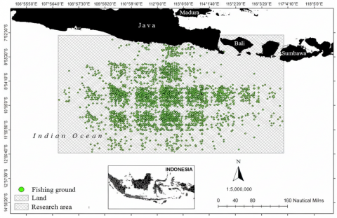
Spatial analysis of logbook records and fisher interviews yielded 5,584 georeferenced points from interviews and 8,213 points from logbooks, delineating tuna fishing grounds between 108°–116° E and 8°–14° S (Figure 1). These grounds extend from approximately 4 nautical miles off the south Java coast to around 325 nautical miles offshore, indicating that both nearshore and distant oceanic habitats of the genus Thunnus are exploited. Most effort clusters along preferred “corridors” aligned with port access from Pondokdadap, reflecting typical patterns seen when fishing grounds are reconstructed from logbooks, VMS, and fisher-reported positions in small-scale and semi-industrial tuna fleets [35-37]. Because fishing range and operational capability can influence where effort occurs, this spatial footprint is interpreted as an effort distribution (opportunity space) rather than a direct map of stock distribution. This footprint forms the basis for subsequent analyses linking fishing locations, oceanographic conditions, and mapped habitat suitability (PHI).
Figure 1. Map of tuna fishing areas in the study region based on logbook and interview data
3.2 Catch composition
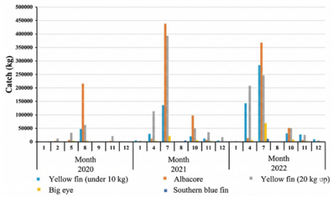
Over the 2020–2022 period, total landings of tuna (genus Thunnus) at Pondokdadap reached 3,421,221 kg, comprising yellowfin, albacore, bigeye, and southern bluefin tuna (Figure 2). These landings summarize port-level production and are influenced by both availability and fishing operations; therefore, they are interpreted alongside effort (trips) and environmental conditions rather than as abundance alone.
Figure 2. Three-year tuna catch production (2020–2022) by weight landed at Pondokdadap
Annual production increased markedly, with the lowest total recorded in 2020 (423,325 kg) and the highest in 2022 (1,574,149 kg). This increase likely reflects a combination of environmental variability and operational factors (e.g., trip intensity, spatial expansion, and fleet behaviour), rather than a simple change in stock size. The pattern is consistent with regional observations that yellowfin, bigeye, and albacore dominate industrial and coastal landings and that their relative contributions can shift with environmental variability and fleet behaviour [21, 38].
3.3 Catch class interval
Monthly tuna catches (kg per month) over three years were grouped into five Sturges-based classes. The data range (271–603,023 kg) and resulting class interval of approximately 120,550 kg produced a highly skewed frequency distribution, with 50% of observations in the lowest class (271–120,821 kg) and 21% in the highest class (482,472–603,023 kg), as shown in Table 1. Intermediate classes were sparsely occupied, including one class with no observations, highlighting the contrast between frequent low-yield months and relatively rare high-production peaks. This descriptive stratification is used to contextualize subsequent CPUE–environment analyses and does not imply discrete regime shifts without additional testing. The approach mirrors standard methods for exploring fisheries time series and identifying dominant production levels and tail events in catch or CPUE data [39, 40].
Table 1. Class intervals, frequencies, and relative frequencies of monthly tuna catches (2020–2022)
|
Class |
Interval (kg) |
Class Interval (kg) |
F |
F(%) |
|
|
1 |
271 |
120,821 |
271-120,821 |
7 |
50 |
|
2 |
120,821 |
241,372 |
120,821-241,372 |
3 |
21 |
|
3 |
241,372 |
361,922 |
241,372-361,922 |
0 |
0 |
|
4 |
361,922 |
482,472 |
361,922-482,472 |
1 |
7 |
|
5 |
482,472 |
603,023 |
482,472-603,023 |
3 |
21 |
|
Total |
14 |
100 |
|||
3.4 Catch per unit effort
CPUE for Thunnus spp. landed by handline and trolling fleets showed pronounced temporal variability. Several months in 2020–2022 recorded CPUE values of 0 kg/trip, reflecting lean seasons and unfavourable weather that restricted operations. The lowest non-zero CPUE occurred in September 2020 (0.6 kg/trip), while the highest was observed in April 2021 (572.9 kg/trip). Because CPUE is expressed as catch-per-trip, it does not account for differences in fishing capacity (e.g., vessel power/tonnage, crew, gear configuration, trip duration), and it can be influenced by fisher behaviour and FAD use. Accordingly, CPUE is treated here as an operational proxy suitable for linking to environmental variability, rather than as a fully standardized abundance index. This limitation is consistent with data-limited tropical tuna fisheries, where methodological consistency, environmental variation, and fleet behaviour condition the interpretation of CPUE-based habitat models [41-43].
3.5 Oceanographic variation
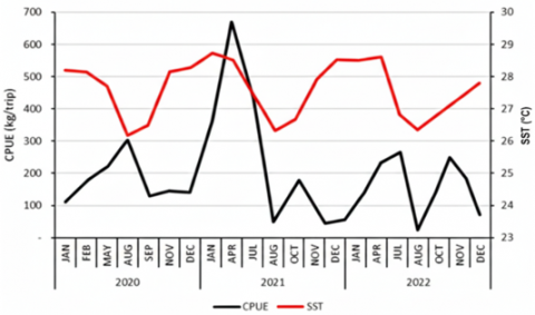
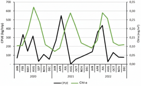
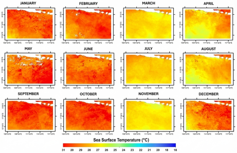
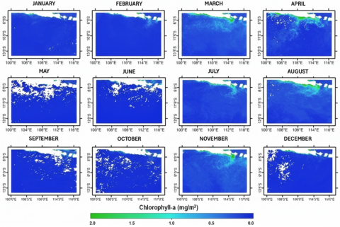
Average SST in the study area over three years was 27.12℃, with values ranging from 25.45℃ (August 2020) to 28.79℃ (February 2020). Mean Chl-a concentration was 0.16 mg m⁻³, varying between 0.06 mg m⁻³ (January 2021) and 0.36 mg m⁻³ (August 2020). To highlight monsoon-driven seasonality, SST and Chl-a are summarized using multi-year monthly (or quarterly) means rather than annual-only panels. These summaries show cooler surfaces and elevated Chl-a during periods aligned with the southeast monsoon, consistent with monsoon-driven upwelling south of Java [44].
(a)
(b)
Figure 4. Annual SST distribution in the study area for 2020-2022
Figure 5. Chlorophyll-a (Chl-a) distribution (in mg/m³) in the study area for 2020-2022
Temporal overlays of catch, SST, and Chl-a (Figure 3) indicate that higher catches often occurred when SST was moderately cool and Chl-a within a moderate range, consistent with monsoon-linked productivity pulses. For example, in August 2020 catches reached 330,865 kg with CPUE 230 kg/trip at SST 25.45℃ and Chl-a 0.31 mg m⁻³, while in July 2022 catches were 979,593 kg with CPUE 428 kg/trip at SST 26.04℃ and Chl-a 0.28 mg m⁻³. These observations are consistent with tropical Indian Ocean studies where cooler, nutrient-enriched surface waters and elevated Chl-a are associated with enhanced tuna productivity and catch peaks [45]. The spatial distribution of SST and Chl-a in the study area for 2020-2022 is shown in Figures 4 and 5.
3.6 Generalized Additive Models analysis
GAMs were fitted to relate the CPUE proxy of Thunnus spp. to SST, Chl-a, and their combination. The SST-only model (SST) produced the lowest Akaike Information Criterion (AIC) (17,342) and explained ~2% of deviance, while the Chl-a model explained ~2.21% of deviance (AIC 17,359). The combined SST + Chl-a model increased deviance explained to ~4.21% but had a higher AIC (17,512), indicating a trade-off between fit and complexity. Although smooth terms were statistically significant (P < 2e-16; Table 2), the overall explanatory power was low, suggesting that substantial variability in CPUE is driven by unmodelled factors (e.g., operational behaviour, fleet heterogeneity, FAD dynamics, and other environmental covariates). Following GAM selection criteria that balance deviance explained and penalize complexity [46, 47], the SST model was retained as the most parsimonious formulation for deriving interpretable habitat windows, while the combined model is reported as an upper bound on fit under the available covariates.
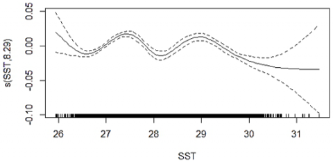
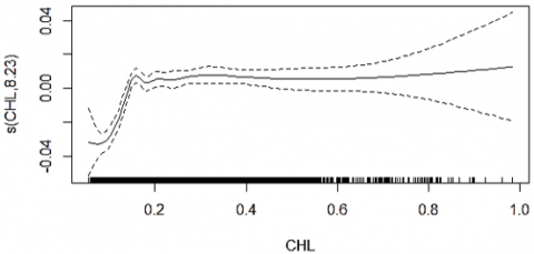
The GAM smoother plots (Figure 6) show that SST values between approximately 26 and 30.5℃ and Chl-a levels around 0.1–0.9 mg m⁻³ contribute positively to CPUE, while values outside these ranges depress predicted catch. These habitat windows are consistent with broader GAM applications where SST, productivity proxies, and depth-related variables emerge as key predictors of pelagic fish distributions and catch variability [48-50].
(a)
(b)
Figure 6. GAM smoothing curves for SST and Chl-a with 95% confidence intervals showing their effects on CPUE
Table 2. GAM model statistics for CPUE as a function of SST, Chl-a, and their combination
|
No. |
Model |
Variable |
P-Value |
DE |
AIC |
edf |
|
1 |
SST |
SST |
<2e-16 *** |
2% |
17342 |
8.287 |
|
2 |
Chlorophyll-a |
Chlorophyll-a |
<2e-16 *** |
2.21% |
17359 |
8.229 |
|
3 |
SST+ Chlorophyll-a |
SST |
<2e-16 *** |
4.21% |
17512 |
8.418 |
|
|
|
Chlorophyll-a |
<2e-16 *** |
|
|
7.523 |
***: p < 0.001.
3.7 Pelagic habitat index analysis
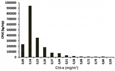
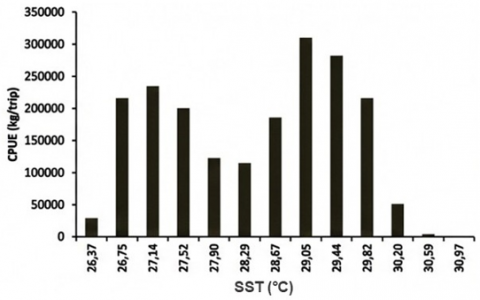
PHI analysis integrated the GAM-derived suitability signal with SST and Chl-a to classify tuna habitat suitability. Histograms of CPUE against SST and Chl-a (Figure 7) show that the highest CPUE (as a catch-per-trip proxy) occurred at SST 28.86–29.25℃ (mean 29.05℃), while the minimum CPUE was associated with the warmest class (30.78–31.16℃, mean 30.97℃). For Chl-a, maximum CPUE occurred at 0.13–0.20 mg m⁻³ (median ~0.16 mg m⁻³), whereas the lowest CPUE was linked to the highest Chl-a class (0.90–0.97 mg m⁻³). These class-based summaries are used to interpret the environmental ranges that dominate observed catches and to support the “habitat window” interpretation from the GAM smoother curves.
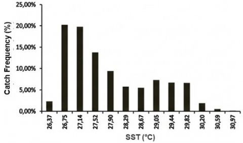
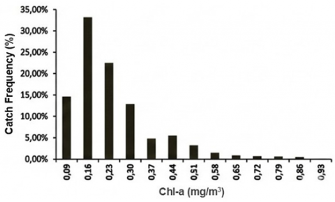
Frequency histograms (Figure 7) demonstrate that most tuna catches were associated with SST 26.37–30.97℃, with the peak frequency (20.25%) in the 26.56–26.95℃ class. For Chl-a, 33.12% of catch frequency fell within 0.13–0.20 mg m⁻³, reinforcing this range as a core productivity window. These patterns are consistent with PHI applications elsewhere, where moderate Chl-a fronts and optimal thermal ranges define medium–high suitability habitats for skipjack and yellowfin tuna [8, 28, 29]. Because the GAM deviance explained is low, these distributions are interpreted as dominant observational regimes rather than deterministic predictors.
(a)
(b)
(c)
(d)
Figure 7. Histograms of (a) CPUE–Chl-a; (b) CPUE–SST; (c) Catch frequency–SST; and (d) Catch frequency–Chl-a
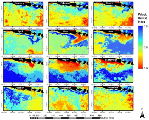
Interpolated PHI values over 2020–2022 ranged from 0 to 1 after normalization (negative values were removed by rescaling the underlying suitability field), and were classified into low, medium, and high potential categories (Figure 8). Classification thresholds were defined explicitly (e.g., quantiles or fixed cut-points), and the rationale for the selected cut-points is reported to ensure reproducibility. Of 97,884 interpolated pixels, 29.47% fell in the low, 59.00% in the medium, and 11.53% in the high potential class. Seasonally, April exhibited the highest number of tuna hauls in the medium class (7,562 hauls; 93%), whereas March contained a small proportion of hauls in the high-potential class (71 hauls; 1%). This dominance of medium-class habitat and the restricted extent of high-PHI cells mirrors other PHI-based studies in tropical tuna grounds, where values above ~0.75 delineate core hotspots within a broader matrix of moderate suitability [29, 51, 52]. To strengthen decision relevance, the monthly PHI maps are additionally summarized by reporting the centroid coordinates and the areal extent of “high” zones, and by filtering zones within a feasible travel distance from the home port to reflect vessel range limits.
Figure 8. Map of pelagic habitat index (PHI) classes (low, medium, high) for Thunnus spp. in the study area (2020–2022)
The SST–Chl-a windows identified in this study (SST≈26–30.5℃; Chl-a≈0.1–0.9 mg m⁻³) are broadly consistent with tuna habitat preferences reported from other regions of the Indian and Pacific Oceans. Skipjack and other tropical tunas in the Makassar Strait, for example, occupy areas with elevated Chl-a and optimal SST ranges, reflecting coupling between primary productivity and pelagic predator distribution [29]. In the southeastern Indian Ocean, albacore tuna shows a narrower thermal niche (15–26℃), highlighting interspecific differences in habitat windows even within the same basin [53]. These comparisons support the ecological plausibility of the identified “windows,” while emphasizing that ranges are species- and region-specific.
Seasonal displacement of skipjack habitats driven by SST and Chl-a gradients [8], resembles the seasonal shift of favourable habitat south of Java observed in our PHI patterns. By contrast, yellowfin tuna often shows more stable thermal preferences modulated by decadal climate variability [54]. These comparisons suggest that our SST–Chl-a windows for Thunnus spp. South of Java aligns with regional patterns while retaining local specificity shaped by monsoon-driven upwelling. The convergence of tuna habitat around moderate SST and enhanced Chl-a reported in Atlantic and Indian Ocean meta-analyses [55] supports the generality of these niches. In this study, the GAM–PHI workflow is used to translate those niches into spatially explicit maps, not to claim real-time predictive forecasting.
Comparative evidence across Pacific–Indian settings reinforces that tuna aggregation is frequently associated with productivity gradients and temperature boundaries, but the exact ranges vary by species and region. Therefore, the “windows” reported here are interpreted as regionally calibrated ranges for southern Java rather than universal constants [8, 29, 53].
The sensitivity of habitat patterns to year-to-year changes in SST and Chl-a is consistent with evidence that ENSO and IOD events modify tuna habitat and CPUE in Indonesian waters. Istnaeni et al. [20] showed that ENSO- and IOD-driven anomalies in SST and Chl-a alter yellowfin presence and catch rates in the eastern Indian Ocean, while Wiryawan et al. [56] linked large yellowfin distribution and CPUE to physical changes in the water column. This context is important because the GAMs in the present study explain only ~2–4% of deviance, indicating that interannual climate variability and operational factors can overwhelm the partial effects of SST and Chl-a in catch-per-trip data.
Incorporating dynamic oceanographic drivers into GAMs has been shown to improve deviance explained and reduce bias for pelagic species [21, 27]. Similarly, changes in primary productivity and upwelling intensity documented by Hsiao et al. [57] suggest that habitat suitability for tuna can move rapidly in space, which challenges static habitat models. Habitat Suitability Index and related indices for Euthynnus affinis have also been shown to track SST and Chl-a changes associated with seasonal upwelling and IOD phases [49], reinforcing the need to interpret PHI and GAM outputs in a climate-contextual framework. At broader scales, long-term projections indicate that ongoing climate change, superimposed on natural variability, will shift tuna habitats and prey fields [58], implying that the environmental windows identified here may change in position and width over the coming decades. This supports treating PHI as a mapping framework that should be recalibrated as new data accumulate, rather than as a fixed “rule”. Given the modest deviance explained (~2–4%), future models should explicitly incorporate climate indices (ENSO/IOD) and additional covariates (e.g., wind-driven upwelling proxies, current strength, mixed-layer depth) to stabilize habitat–catch relationships across years [20, 27, 56, 56].
In practical fisheries governance, GAM and PHI-based habitat products can support ecosystem-based fisheries management (EBFM) and spatial planning by providing routinely updated (e.g., monthly) habitat suitability maps that identify “high suitability” zones and their geographic coordinates. In the context of this study, implementation would involve: (i) producing a monthly PHI map, (ii) delineating polygons/cells classified as “high,” (iii) reporting their centroid coordinates and areal extent, and (iv) filtering candidate zones by feasible travel distance from the home port to reflect vessel range and safety constraints. These map-based outputs can then inform seasonal spatial prioritization (e.g., voluntary effort concentration, monitoring focus, or time–area planning) and, where governance capacity exists, can be considered alongside conservation objectives (e.g., bycatch risk periods) [59-62]. Because the present work is based on historical data and exhibits modest explanatory power, claims of “near-real-time advisories” are avoided; the contribution is a transparent framework for generating spatial habitat suitability products.
Future extensions can integrate climate indices (ENSO/IOD) and operational constraints (vessel capability, safety, costs) into a multi-criteria habitat suitability and planning framework to improve robustness across years. Including simple effort-capacity covariates (e.g., vessel class/GT, engine power, gear specifications) would also address limitations of catch-per-trip CPUE and may increase explanatory power. Such integration would strengthen PHI as an adaptive planning instrument under climate-driven variability.
From a design perspective, this study translates remotely sensed ocean dynamics into an operational habitat indicator (PHI) that supports interpretable, map-based decision-making in tuna fisheries. By converting environmental variability into spatially explicit habitat suitability information, the framework enables oceanographic signals to be interpreted for management and operational planning. Indicator-based approaches such as PHI provide a bridge between environmental monitoring and applied fisheries governance. In this study, the actionable output is the generation of monthly or seasonal habitat suitability maps (low–medium–high) and the delineation of recurrent high-suitability zones, rather than real-time forecasting or prescriptive “advisories.” This design-oriented interpretation highlights remote sensing not only as a descriptive tool, but as a foundation for developing replicable planning instruments that can support efficient and risk-aware fisheries management under monsoon-driven variability.
This study demonstrates that satellite-derived ocean dynamics can be translated into spatially explicit habitat suitability maps through an indicator-based eco-informatics framework. The most critical results indicate that tuna catches are associated with SST ≈26–30.5℃ and Chl-a ≈ 0.1–0.9 mg m⁻³, and that PHI maps highlight recurrent medium–high suitability zones in the study area across monsoon phases. The GAM component shows modest explanatory power (~2–4% deviance explained), indicating that suitability patterns should be interpreted as partial habitat signals conditioned on limited covariates and simplified effort standardization. By integrating SST and Chl-a within a GAM and operationalizing fitted responses into PHI classes, complex ecological relationships are transformed into interpretable spatial products.
The findings highlight that, despite heterogeneous fishing behaviour and climate-driven variability, indicator-based habitat mapping provides a structured basis for seasonal spatial planning. Rather than claiming efficiency gains directly, the framework offers a transparent method to delineate candidate “high suitability” zones that can inform fishing-ground selection, monitoring focus, and spatial planning under ecosystem-based fisheries management objectives.
This study contributes to the existing body of knowledge by shifting habitat modelling from descriptive analysis toward map-based decision support, emphasizing the role of indicators in linking ocean dynamics to fisheries governance. Future research should incorporate climate indices (ENSO/IOD), effort-capacity covariates (vessel/gear characteristics), and operational constraints (range, safety, cost) to strengthen multi-criteria planning tools under increasing environmental variability.
The authors gratefully acknowledge the financial support provided by Universitas Brawijaya through the Dosen Berkarya Grant. The authors also appreciate the research collaboration with the Department of Technology and Industrial, Faculty of Science and Technology, Prince of Songkla University, Thailand, which contributed to academic discussions and knowledge exchange supporting this study.
[1] Ningsih, W.A.L., Lestariningsih, W.A., Heltria, S., Khaldun, M.H.I. (2021). Analysis of the relationship between chlorophyll-a and sea surface temperature on marine capture fisheries production in Indonesia: 2018. IOP Conference Series: Earth and Environmental Science, 944(1): 012057. https://doi.org/10.1088/1755-1315/944/1/012057
[2] Hidayat, A.S., Rajiani, I., Arisanty, D. (2022). Sustainability of floodplain wetland fisheries of rural Indonesia: Does culture enhance livelihood resilience?. Sustainability, 14(21): 14461. https://doi.org/10.3390/su142114461
[3] Sari, Q.W., Siswanto, E., Utari, P.A., Saputra, O.F., et al. (2022). Seasonal driven mechanism of the surface chlorophyll-a distribution along the Western Coast of Sumatra. Journal of Ecological Engineering, 23(11): 254-260. https://doi.org/10.12911/22998993/153995
[4] Suharyanto, S., Gunaisah, E., Katili, V.R., Dewi, P., et al. (2022). Effect of sea surface temperature and chlorophyll-a on the total catches of lift net fishery in the Padang Pariaman Regency, Indonesia. Jurnal Airaha, 11(2): 253-266. https://doi.org/10.15578/ja.v11i02.349
[5] Prasetya, M.R., Avrionesti, A., Haryanto, Y.D., Qomariyatuzzamzami, L.N. (2024). The identification of upwelling in the occurrence of tropical cyclone charlotte in the waters of Southern Java (Case study: March 17-28, 2022). Tropical Marine Environmental Sciences, 2(2): 30-35. https://doi.org/10.31258/tromes.2.2.30-35
[6] Suprianto, A., Atmadipoera, A.S., Lumban-Gaol, J. (2021). Seasonal coastal upwelling in the Bali Strait: A model study. IOP Conference Series: Earth and Environmental Science, 944(1): 012055. https://doi.org/10.1088/1755-1315/944/1/012055
[7] Horii, T., Ueki, I., Syamsudin, F., Sofian, I., Ando, K. (2016). Intraseasonal coastal upwelling signal along the southern coast of Java observed using Indonesian tidal station data. Journal of Geophysical Research: Oceans, 121(4): 2690-2708. https://doi.org/10.1002/2015jc010886
[8] Mugo, R., Saitoh, S.I., Igarashi, H., Toyoda, T., Masuda, S., Awaji, T., Ishikawa, Y. (2020). Identification of skipjack tuna (Katsuwonus pelamis) pelagic hotspots applying a satellite remote sensing-driven analysis of ecological niche factors: A short-term run. PloS One, 15(8): e0237742. https://doi.org/10.1371/journal.pone.0237742
[9] Zainuddin, M., Amir, M.I., Bone, A., Farhum, S.A., et al. (2019). Mapping distribution patterns of skipjack tuna during January-May in the Makassar Strait. IOP Conference Series: Earth and Environmental Science, 370(1): 012004. https://doi.org/10.1088/1755-1315/370/1/012004
[10] Kareem, H.H., Attaee, M.H., Omran, Z.A. (2023). Extraction of the spatial and temporal surface water bodies using high resolution remote sensing technology at Cardiff City, United Kingdom. Journal of Ecological Engineering, 24(11): 135-147. https://doi.org/10.12911/22998993/171543
[11] Sachoemar, S.I., Yanagi, T., Aliah, R.S. (2012). Variability of sea surface chlorophyll-a, temperature and fish catch within Indonesian region revealed by satellite data. Marine Research in Indonesia, 37(2): 75-87. https://doi.org/10.14203/mri.v37i2.25
[12] Manik, A., Arifuddin, A.M.N., Pawara, M.U., Nurcholik, S.D., Ikhwani, R.J. (2023). Analysis of gross tonnage (GT) capacity installed on traditional wooden ships in Penajam Paser Utara. Indonesian Journal of Maritime Technology, 1(2): 78-84. https://doi.org/10.35718/ismatech.v1i2.1059
[13] Rahman, H., Abidin, R.Z., Hidayat, N. (2025). Analysis of the economic potential of the marine capture fisheries sector in Sumenep regency with gordon-schaefer model approach. IOP Conference Series: Earth and Environmental Science, 1454(1): 012038. https://doi.org/10.1088/1755-1315/1454/1/012038
[14] Widodo, A.A., Wudianto, W., Sadiyah, L., Mahiswara, M., Proctor, C., Cooper, S. (2020). Investigation on tuna fisheries associated with fish aggregating devices (FADs) in Indonesia FMA 572 and 573. Indonesian Fisheries Research Journal, 26(2): 83-96. https://doi.org/10.15578/ifrj.26.2.2020.83-96
[15] Widodo, M.P., Idris, I., Aprilya, N., Fakhrurrozi, F., et al. (2023). Analysis of the suitability and carrying capacity of marine and coastal tourism on Tunda Island, Banten Province. BIO Web of Conferences, 70: 06008. https://doi.org/10.1051/bioconf/20237006008
[16] Andrimida, A., Wiadnya, D.G.R., Hardiyan, F.Z. (2022). New record of the Armored Gurnard Satyrichthys laticeps (Schlegel, 1852) (Scorpaeniformes: Peristediidae) from Java South Sea (Eastern Indian Ocean). Indo Pacific Journal of Ocean Life, 6(2): 74-79. https://doi.org/10.13057/oceanlife/o060202
[17] Barclay, K.M., Satapornvanit, A.N., Syddall, V.M., Williams, M.J. (2022). Tuna is women's business too: Applying a gender lens to four cases in the Western and Central Pacific. Fish and Fisheries, 23(3): 584-600. https://doi.org/10.1111/faf.12634
[18] Rahayu, T., Yusriadi, Y., Kusumawati, E., Eddi, E., Pribadi, T. (2025). The role of coastal fisheries infrastructure in enhancing food security: A case study of Mayangan port. African Journal of Food Agriculture Nutrition and Development, 25(6): 26879-26899. https://doi.org/10.18697/ajfand.143.25725
[19] Amri, K., Suman, A., Irianto, H.E., Wudianto, W. (2015). Effects of dipole mode and El-nino events on catches of yellowfin tuna (Thunnus albacares) in the eastern Indian ocean off west java. Indonesian Fisheries Research Journal, 21(2): 75-90. https://doi.org/10.15578/ifrj.21.2.2015.75-90
[20] Istnaeni, Z.D., Hidayat, R., Zainuddin, M., Gaol, J.L., Fitrianah, D. (2024). The ENSO-IOD effects on Yellowfin tuna (Thunnus albacares) in Eastern Indian Ocean-Off Coast Java. IOP Conference Series: Earth and Environmental Science, 1410(1): 012043. https://doi.org/10.1088/1755-1315/1410/1/012043
[21] Sambah, A.B., Noor’izzah, A.U.R.U.M., Intyas, C.A., Widhiyanuriyawan, D., Affandy, D.P., Wijaya, A.D.I. (2023). Analysis of the effect of ENSO and IOD on the productivity of yellowfin tuna (Thunnus albacares) in the South Indian Ocean, East Java, Indonesia. Biodiversitas Journal of Biological Diversity, 24(5): 2689-2700. https://doi.org/10.13057/biodiv/d240522
[22] Nataniel, A., Pennino, M.G., Lopez, J., Soto, M. (2022). Modelling the impacts of climate change on skipjack tuna (Katsuwonus pelamis) in the Mozambique Channel. Fisheries Oceanography, 31(2): 149-163. https://doi.org/10.1111/fog.12568
[23] Nicol, S., Lehodey, P., Senina, I., Bromhead, D., et al. (2022). Ocean futures for the world’s largest yellowfin tuna population under the combined effects of ocean warming and acidification. Frontiers in Marine Science, 9: 816772. https://doi.org/10.3389/fmars.2022.816772
[24] Zhang, Y., Lun, H. (2023). Remote sensing and image processing techniques for water environment monitoring: A case study of the Beijing-Tianjin-Hebei region. Traitement du Signal, 40(4): 1771-1779. https://doi.org/10.18280/ts.400447
[25] Indriyani, L., Kete, S.C.R., Isabela, Fitriani, V., Gandri, L., De Ahmaliun, L. (2025). Impacts of vegetation dynamics on land surface temperature and moisture in Kendari City, Indonesia: A remote sensing study. International Journal of Design & Nature and Ecodynamics, 20(10): 2315-2323. https://doi.org/10.18280/ijdne.201010
[26] Mohammed, M.B., Baba, I.A., Salihu, H.D., Ibrahim, I.A. (2025). New class width rule for continuous frequency tables. Results in Control and Optimization, 18: 100506. https://doi.org/10.1016/j.rico.2024.100506
[27] Hasyim, S., Hidayat, R., Farhum, S.A., Zainuddin, M. (2022). The use of statistical models in identifying skipjack tuna habitat characteristics during the Southeast Monsoon in the Bone Gulf, Indonesia. Biodiversitas Journal of Biological Diversity, 23(4): 2231-2237. https://doi.org/10.13057/biodiv/d230459
[28] Zainuddin, M., Farhum, A., Safruddin, S., Selamat, M.B., et al. (2017). Detection of pelagic habitat hotspots for skipjack tuna in the Gulf of Bone-Flores Sea, southwestern Coral Triangle tuna, Indonesia. PLoS One, 12(10): e0185601. https://doi.org/10.1371/journal.pone.0185601
[29] Hidayat, R., Zainuddin, M., Mallawa, A., Mustapha, M.A., Putri, A.R.S. (2021). Mapping spatial-temporal skipjack tuna habitat as a reference for Fish Aggregating Devices (FADs) settings in Makassar Strait, Indonesia. Biodiversitas Journal of Biological Diversity, 22(9): 3637-3647. https://doi.org/10.13057/biodiv/d220905
[30] Pane, A.R.P., Alnanda, R., Prihatiningsih, P., Hufiadi, H., Suman, A. (2020). The fishing ground of bottom longline vessels and exploitation rate of tiger grouper (Epinephelus aerolatus) in Arafura Waters. Omni-Akuatika, 16(3): 33-41. https://doi.org/10.20884/1.oa.2020.16.3.850
[31] Zainuddin, M., Safruddin, S., Farhum, A., Budimawan, B., et al. (2023). Satellite-Based ocean color and thermal signatures defining habitat hotspots and the movement pattern for commercial skipjack tuna in Indonesia Fisheries Management Area 713, Western Tropical Pacific. Remote Sensing, 15(5): 1268. https://doi.org/10.3390/rs15051268
[32] Adiputra, R.M.C.S., Djunarsjah, E., Muharram, F.W., Putra, A.P. (2025). Spatial analysis of potential fishing zones (PFZ) for tuna in Parangtritis waters based on sea surface temperature, chlorophyll-a, and bathymetry. Jurnal Komputer Teknologi Informasi Sistem Informasi (JUKTISI), 4(2): 531-545. https://doi.org/10.62712/juktisi.v4i2.470
[33] Rifki, R.A., Chairani, C., Sriyanto, S. (2025). Utilization of satellite imagery and GIS for mapping potential anchovy fishing areas in east Lampung. Inovtek Polbeng-Seri Informatika, 10(2): 784-795. https://doi.org/10.35314/t4fqfq25
[34] Vaihola, S., Yemane, D., Kininmonth, S. (2023). Spatiotemporal patterns in the distribution of albacore, bigeye, skipjack, and yellowfin tuna species within the exclusive economic zones of Tonga for the years 2002 to 2018. Diversity, 15(10): 1091. https://doi.org/10.3390/d15101091
[35] Cimino, M.A., Anderson, M., Schramek, T., Merrifield, S., Terrill, E.J. (2019). Towards a fishing pressure prediction system for a western Pacific EEZ. Scientific Reports, 9(1): 461. https://doi.org/10.1038/s41598-018-36915-x
[36] Natale, F., Gibin, M., Alessandrini, A., Vespe, M., Paulrud, A. (2015). Mapping fishing effort through AIS data. PloS One, 10(6): e0130746. https://doi.org/10.1371/journal.pone.0130746
[37] Watson, J.T., Haynie, A.C. (2016). Using vessel monitoring system data to identify and characterize trips made by fishing vessels in the United States North Pacific. PloS One, 11(10): e0165173. https://doi.org/10.1371/journal.pone.0165173
[38] Sukresno, B., Hartoko, A., Sulistyo, B. (2015). Empirical cumulative distribution function (ECDF) analysis of thunnus. sp using ARGO float sub-surface multilayer temperature data in Indian Ocean south of java. Procedia Environmental Sciences, 23: 358-367. https://doi.org/10.1016/j.proenv.2015.01.052
[39] Abdellaoui, B., Berraho, A., Falcini, F., Santoleri, J.R., Sammartino, M., Pisano, A., Hilm, K. (2017). Assessing the impact of temperature and chlorophyll variations on the fluctuations of sardine abundance in Al-Hoceima (South Alboran Sea). Journal of Marine Science: Research & Development, 7(4): 1-11. https://doi.org/10.4172/2155-9910.1000239
[40] Owiredu, S.A., Onyango, S.O., Song, E.A., Kim, K.I., Kim, B.Y., Lee, K.H. (2024). Enhancing chub mackerel catch per unit effort (CPUE) standardization through high-resolution analysis of Korean large purse seine catch and effort using AIS data. Sustainability, 16(3): 1307. https://doi.org/10.3390/su16031307
[41] Irham, M., Akbar, M.W., Mukhli, M., Fuadi, A., Authar, M., Setiawan, I. (2022). Catching investigation of yellowfin tuna (Thunnus Albacares) based on the distribution of chlorophyll-a in the North Waters of Aceh: A November and December analysis. E3S Web of Conferences, 339: 02004. https://doi.org/10.1051/e3sconf/202233902004
[42] Martínez-Ortiz, J., Aires-da-Silva, A.M., Lennert-Cody, C.E., Maunder, M.N. (2015). The Ecuadorian artisanal fishery for large pelagics: Species composition and spatio-temporal dynamics. PloS One, 10(8): e0135136. https://doi.org/10.1371/journal.pone.0135136
[43] Stompe, D.K., Roberts, J.D., Estrada, C.A., Keller, D.M., Balfour, N.M., Banet, A.I. (2020). Sacramento River predator diet analysis: A comparative study. San Francisco Estuary and Watershed Science, 18(1): 1-16. https://doi.org/10.15447/sfews.2020v18iss1art4
[44] Gao, G., Yang, D., Xu, L., Zhang, K., Feng, X., Yin, B. (2022). A biological-parameter-optimized modeling study of physical drivers controlling seasonal chlorophyll blooms off the southern coast of Java Island. Journal of Geophysical Research: Oceans, 127(11): e2022JC018835. https://doi.org/10.1029/2022jc018835
[45] Kong, F., Dong, Q., Xiang, K., Yin, Z., Li, Y., Liu, J. (2019). Spatiotemporal variability of remote sensing ocean net primary production and major forcing factors in the Tropical Eastern Indian and Western Pacific Ocean. Remote Sensing, 11(4): 391. https://doi.org/10.3390/rs11040391
[46] Roberts, S.M., Boustany, A.M., Halpin, P.N. (2020). Substrate-dependent fish have shifted less in distribution under climate change. Communications Biology, 3(1): 586. https://doi.org/10.1038/s42003-020-01325-1
[47] Zieritz, A., Bogan, A.E., Rahim, K.A.A., Sousa, R., et al. (2018). Changes and drivers of freshwater mussel diversity and distribution in northern Borneo. Biological Conservation, 219: 126-137. https://doi.org/10.1016/j.biocon.2018.01.012
[48] Houssard, P., Point, D., Tremblay-Boyer, L., Allain, V., et al. (2019). A model of mercury distribution in tuna from the western and central Pacific Ocean: Influence of physiology, ecology and environmental factors. Environmental Science & Technology, 53(3): 1422-1431. https://doi.org/10.1021/acs.est.8b06058
[49] Koropitan, A.F., Kholilullah, I., Yusfiandayani, R. (2021). Modeling mackerel tuna (Euthynnus affinis) habitat in southern coast of Java: Influence of seasonal upwelling and negative IOD. HAYATI Journal of Biosciences, 28(4): 271-285. https://doi.org/10.4308/hjb.28.4.271-285
[50] Mondal, S., Ray, A., Osuka, K.E., Sihombing, R.I., Lee, M.A., Chen, Y.K. (2023). Impact of climatic oscillations on marlin catch rates of Taiwanese long-line vessels in the Indian Ocean. Scientific Reports, 13(1): 22438. https://doi.org/10.1038/s41598-023-49984-4
[51] Arnenda, G.L., Rochman, F., Wujdi, A., Kurniawan, R. (2021). Estimated production, catch per unit effort, biological aspects of tuna, skipjack, and small tuna in North Sumatra. E3S Web of Conferences, 322: 03003. https://doi.org/10.1051/e3sconf/202132203003
[52] Lezama-Ochoa, N., Murua, H., Ruiz, J., Chavance, P., Delgado de Molina, A., Caballero, A., Sancristobal, I. (2018). Biodiversity and environmental characteristics of the bycatch assemblages from the tropical tuna purse seine fisheries in the eastern Atlantic Ocean. Marine Ecology, 39(3): e12504. https://doi.org/10.1111/maec.12504
[53] Nugroho, S.C., Setiawan, R.Y., Setiawati, M.D., Priyono, S.B., Susanto, R.D., Wirasatriya, A., Larasati, R.F. (2022). Estimation of albacore tuna potential fishing grounds in the southeastern Indian Ocean. IEEE Access, 11: 1141-1147. https://doi.org/10.1109/access.2022.3233353
[54] Wu, Y.L., Lan, K.W., Evans, K., Chang, Y.J., Chan, J.W. (2022). Effects of decadal climate variability on spatiotemporal distribution of Indo-Pacific yellowfin tuna population. Scientific Reports, 12(1): 13715. https://doi.org/10.1038/s41598-022-17882-w
[55] Druon, J.N., Chassot, E., Murua, H., Lopez, J. (2017). Skipjack tuna availability for purse seine fisheries is driven by suitable feeding habitat dynamics in the Atlantic and Indian Oceans. Frontiers in Marine Science, 4: 315. https://doi.org/10.3389/fmars.2017.00315
[56] Wiryawan, B., Loneragan, N., Mardhiah, U., Kleinertz, S., et al. (2020). Catch per unit effort dynamic of yellowfin tuna related to sea surface temperature and chlorophyll in Southern Indonesia. Fishes, 5(3): 28. https://doi.org/10.3390/fishes5030028
[57] Hsiao, C.Y., Kuo, C.M., Tuan, C.L. (2021). Island ecological tourism: Constructing indicators of the tourist service system in the Penghu national scenic area. Frontiers in Ecology and Evolution, 9: 708344. https://doi.org/10.3389/fevo.2021.708344
[58] Erauskin-Extramiana, M., Arrizabalaga, H., Hobday, A.J., Cabré, A., et al. (2019). Large-scale distribution of tuna species in a warming ocean. Global Change Biology, 25(6): 2043-2060. https://doi.org/10.1111/gcb.14630
[59] Dunn, D.C., Maxwell, S.M., Boustany, A.M., Halpin, P.N. (2016). Dynamic ocean management increases the efficiency and efficacy of fisheries management. Proceedings of the National Academy of Sciences, 113(3): 668-673. https://doi.org/10.1073/pnas.1513626113
[60] Poulton, A.J., Sethi, S.A., Ellner, S.P., Smeltz, T.S. (2023). Optimal dynamic spatial closures can improve fishery yield and reduce fishing-induced habitat damage. Canadian Journal of Fisheries and Aquatic Sciences, 80(6): 893-912. https://doi.org/10.1139/cjfas-2022-0198
[61] Pons, M., Watson, J.T., Ovando, D., Andraka, S., et al. (2022). Trade-offs between bycatch and target catches in static versus dynamic fishery closures. Proceedings of the National Academy of Sciences, 119(4): e2114508119. https://doi.org/10.1073/pnas.2114508119
[62] Bastardie, F., Astarloa, A., Binch, L., Bitetto, I., et al. (2025). Anticipating how spatial fishing restrictions in EU waters perform to protect marine species, habitats, and dependent fisheries. Frontiers in Marine Science, 12: 1629180. https://doi.org/10.3389/fmars.2025.1629180