Mohammad Radzif Taharin | Rodeano Roslee*
© 2021 IIETA. This article is published by IIETA and is licensed under the CC BY 4.0 license (http://creativecommons.org/licenses/by/4.0/).
OPEN ACCESS
Ordinary Kriging (OK) is one of the geostatistical methods, which were used in the variation types of mapping, which related to the soil. Compliment by semi variogram models, OK has become one of the most sought out method for the digital mapping, which applied Geographical Information System (GIS) as a main approach. Four semi variogram models, which are spherical, exponential, circular and gaussian would be applied to determine the best model for the mapping purposes, with Root-Mean-Squared-Error (RMSE) as a performance indicator. The value of the cohesion and clay percentage will be based according to the related depth. Each semi variogram model will be applied to determine the best model for each depth, whether it is cohesion or clay percentage, and producing a map, as a result. This mapping would be an alternative to the geological mapping, whereby it would show the range of the cohesion and clay percentage values rather than soil types.
Ordinary Kriging, semi variogram, cohesive soil, Sabah
Geostatistical modelling is the latest approach, which were used in the variation types of mapping, related to the soil [1]. Compliment by semi variogram, methods such as Kriging has become one of the most sought out method for the digital mapping, which applied Geographical Information System (GIS) as a main approach. Soil cohesion and clay percentage are related, due to the nature of the clay is cohesive, and it is measured by cohesion value and plasticity index [2]. High cohesion values would contribute to high shear strength of soil, which could indicate the ground stability of the area. The introduction of the new approach, which combined the statistical method and current soil investigation method, could contribute in describing the actual condition of the study area, in a practically visible way [3]. With these results, the area comprises low or high values of related parameters are easily identified. Any actions that need to be taken to address problems occurred from this area could be done in a more convenient way [4].
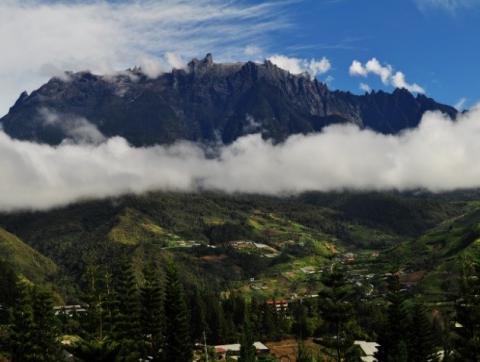
Kundasang, Sabah (Figure 1) has been known for the highland tourism in Malaysia, especially for the Mount Kinabalu, which heights is 4095.2 meters above sea level. This area is popular due to its topography and cool climate, which contributes to the crops production such as vegetables and fruits, and dairy products. Despite blessed with the serene environment, this area is susceptible to the geohazard such as soil mass movements and landslides, which were occurred in high frequency [5-12].
Figure 1. Location of Kundasang area, Sabah, Malaysia
Figure 2. Boreholes location in Kundasang (blue and yellow circle)
Located on two formations, which are Crocker Formation, and Trusmadi Formations, soil in Kundasang is known for low cohesion and high angle of internal friction values. Since cohesion value is usually associated with clay, it is essential to determine the clay percentage distribution of the area, to get the actual view of one of the soil properties. This study would determine the clay percentage distribution for 70 boreholes (Figure 2), from ground level towards 10 meters depth, divided into four equal sections, which are 0 to 2.5 meters, 2.5 to 5 meters, 5 to 7.5 meters, and 7.5 to 10 meters.
Kriging methods (Figure 3) were found by D.G. Krige, in 1953, where the prediction is needed to identify which area has the highest calorie of coal content and the prediction made is showing 96% of accuracy [13]. Expanded by George Matheron, Kriging has become very popular and being used for many purposes, which includes earth science, engineering, medical and vector diseases control [14].
Figure 3. Prediction using ordinary kriging method
$Z=\mu+\varepsilon(\mathrm{s})$ (1)
where,
Z (s)= value that need to be obtained,
$\mu$= mean or the average value that need to be found,
$\varepsilon(\mathrm{s})$= random error which will reduce the value error, which is ±1.96 multiple by kriging error.
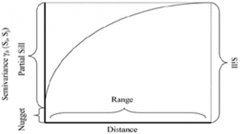
There are several types of Kriging methods, namely Ordinary Kriging, Simple Kriging, Universal Kriging, Indicator Kriging, Disjunctive Kriging, Probability Kriging and Cokriging. But due to its simplicity and accuracy, the Ordinary Kriging (OK) has become the most popular choice [15]. Before OK method could be applied, semivariogram (Figure 4) would be developed to determine the best model for each depth sections, which would be processed for the mapping development of cohesion and clay percentage.
Figure 4. Semivariogram, which comprised of nugget, range and sill
$\gamma(h)=\frac{1}{2} \sum_{i=1}^{n}\left[z\left(x_{i}\right)-z\left(x_{j}+h\right)\right]^{2}$ (2)
where,
$\gamma$ (h)= semivariance between point xi and xj discrete by lag distance h;
n = numbers of pairs of sample points separated by distance h;
z = Attribute value (depends on the parameter that used for this method).
h = distance separating xi and xj.
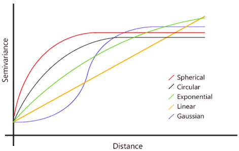
Semivariogram modelling is a key step between spatial description and spatial prediction, which is produced through the least square fit of the data. Four models of semivariogram that would be used in this study are spherical, exponential, circular, and Gaussian (Figure 5). These semivariogram models have different criteria and shape, according to their respective equation [16]. In manual process, the semivariogram calculation would proceed prior to the OK. However, when the calculation is executed by using ArcGIS software, the method have to be selected first due to the variety of Kriging methods availability. Hence, Figure 6 is showing how the process would be executed. The lowest performance indicators value, which is in this case, Root-Mean-Square-Error (RMSE), would be applied as the selected models before proceed to the mapping process.
Figure 5. Types of semivariogram models used for this study
Figure 6. Flowchart showing the methodology used in this study
Prior to the process above, satellite image from JUPEM need to be obtained, together with the borelog of this area. Data of soil cohesion and clay percentage would be produced, provided with the Global Positioning System (GPS) coordinate, together with the associated depth. Different borehole would represent different depth for this study. Analysis will be made once the data have been selected, according to the Kriging methods and semivariogram models. Several graphs and summaries would be displayed prior to the mapping image, such as predicted error, standardized error, and Quantile to Quantile (QQ) plot. Higher accuracy mapping could be produced with higher number of data, since geostatistical mapping is basically based on interpolation [17].
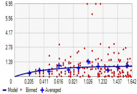
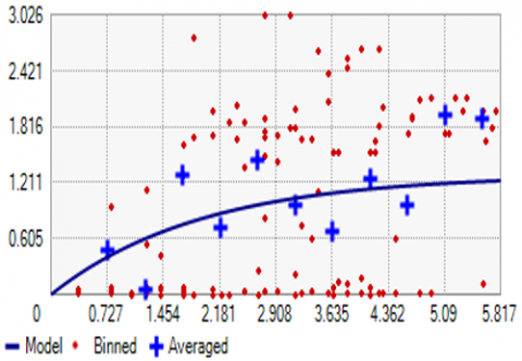
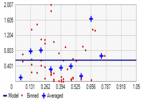
Figure 7 is showing the selected semivariogram according to the depth section for soil cohesion. Circular model emerged as the best model for the depth of 0 – 2.5 meters (Figure 7a), comprising RMSE value of 4.1071. Exponential model standout twice for both depth 2.5 – 5 meters (Figure 7b) and 5 – 7.5 meters (Figure 7c), distinguished by RMSE values of 2.6789 and 2.4425. While for depth 7.5 – 10 meters, any model (Figure 7d) could be selected due to the similar value of RMSE, 2.4176.
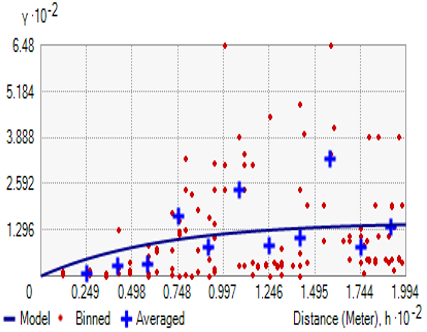
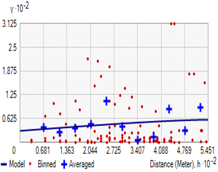
Selected semivariogram for clay percentage distribution is shown in Figure 8. Once again, exponential model standout twice as the best model but for different depth compared to the soil cohesion in Figure 7. Comprising RMSE value of 9.5761 and 5.0340, exponential model is selected for both depth 0 – 2.5 meters (Figure 8a) and 7.5 to 10 meters (Figure 8d). For depth 2.5 – 5 meters and 5 – 7.5 meters, spherical model and circular model have been selected, due to the RMSE values of 9.0670 (Figure 8b) and 6.4173 (Figure 8c). All semivariogram models which has been highlighted here would be selected for the mapping purposes.
(a)
(b)
(c)
(d)
Figure 7. Semi variogram models for soil cohesion, a. Circular, b. Exponential, c. Exponential, d. All models
Figure 9 is showing the mapping of the soil cohesion, for each depth section. For depth 0 to 2.5 meters, high cohesion values could be seen on the top half of the study area, leaving low cohesion values remained in the southeast area and little bit of southwest area (Figure 9a). For depth 2.5 to 5 meters, opposite to the previous depth, low cohesion values dominate the top half of the area, and leave high cohesion values remained at east, southeast, and some in the middle west (Figure 9b). For depth 5 to 7.5 meters, low cohesion values dominated the northwest and middle north area, while high cohesion values dominated the southeast area, leaving the middle area with the intermediate values (Figure 9c). For the final depth, low cohesion values located at middle to southwest area, high cohesion values were dominating west and east area, leaving the middle area with intermediate cohesion values (Figure 9d). It could be seen from Figure 9, that each depth provides different cohesion values, despite separated by 2.5 meters depth.
(a)
(b)
(c)
(d)
Figure 8. Semivariogram models for clay percentage, a. Exponential, b. Spherical, c. Circular, d. Exponential
Figure 9. Cohesion mapping for each depth, a. 0 – 2.5 meters, b. 2.5 – 5 meters, c. 5 – 7.5 meters, d. 7.5 – 10 meters
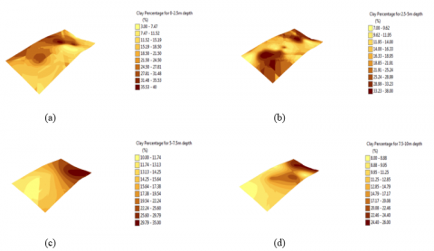
Figure 10. Clay percentage mapping for each depth, a. 0 – 2.5 meters, b. 2.5 – 5 meters, c. 5 – 7.5 meters, d. 7.5 – 10 meters
Figure 10 is showing the mapping of the clay percentage, for each depth section. For depth 0 to 2.5 meters, high clay percentage values could be seen on the top half of the study area, leaving low clay percentage values remained in the west and bottom half area (Figure 10a). For depth 2.5 to 5 meters, low clay percentage values dominate from northwest to southeast of the area, and leave high clay percentage values remained at southwest, northeast, and some in the middle west (Figure 10b). For depth 5 to 7.5 meters, low clay percentage values dominated the northwest and middle north area, while high clay percentage values dominated the southeast area, leaving the middle area with the intermediate values (Figure 10c). For the final depth, low clay percentage values dominated most of the area, leaving high clay percentage values at east area, leaving the middle area with intermediate values (Figure 10d). Similar to Figure 9, Figure 10 is also showing that each depth provides different clay percentage values, despite separated by 2.5 meters depth.
By observing both Figure 9 and Figure 10, it could be found that there are similarities of location between cohesion and clay percentage in both mappings. Both figures are showing high cohesion values are located almost similar to the high clay percentage values and vice versa, according to the depth section. Significantly, most area were dominated by low clay percentage values, which contributed to the low cohesion values. Through this mapping, it could be confirmed that the Kundasang area are suffering from low soil cohesion values and low clay percentage, which is highly exposed and prone to the geohazard disaster such as soil mass movement and landslides.
The application of semivariogram and Ordinary Kriging provide new insight on how soil cohesion and clay percentage could be studied on-site. Furthermore, it could show how these parameters and unit could be related. Lowest RMSE values such as 4.1071. 2.6789, 2.4425, and 2.4176 across all four depths for soil cohesion, and 9.5761, 9.0670, 6.4173 and 5.0340 for clay percentage could contribute in developing digital mapping. Changes in clay percentage could contribute in changes of soil cohesion, which is crucial for ground deformation and landslides. By obtaining these mapping, lots of improvements and remedial works could be planned within this area. These approaches could help the designers, researchers, and other stakeholder (local authority) to make decisions for future developments and geohazard precautions.
Sincere gratitude to Universiti Malaysia Sabah (UMS) for providing easy access to laboratories and research equipment. Highest appreciations also to the research grants award (SDK0012-2017 and SDK0130-2020) to finance all the costs of this research.
[1] Al-Ani, H., Oh, E., Eslami-Andargoli, L., Chai, G. (2013). Subsurface visualization of peat and soil by using GIS in Surfers Paradise, Southeast Queensland, Australia. Electronic Journal of Geotechnical Engineering, 18: 1761-1774.
[2] Brevik, E.C., Hartemink, A.E. (2013). A brief history of soil mapping and classification in the USA. Soil Science Society of America Journal, 77: 1117-1132. https://doi.org/10.2136/sssaj2012.0390
[3] Sabrina, C.Y., Satyanaga, A., Rahardjo, H. (2021). Spatial variation of shear strength properties incorporating auxiliary variables. Catena, 200: 105196. https://doi.org/10.1016/j.catena.2021.105196
[4] Qiao, G., Lu, P., Scaioni, M., Xu, S., Tong, X., Feng, T., Wu, H., Chen, W., Tian, Y., Wang, W., Li, R. (2013). Landslide investigation with remote sensing and sensor network. Remote Sensing, 2013(5): 4319-4346. https://doi.org/10.3390/rs5094319
[5] Simon, N., Roslee, R., Marto, N.L., Akhir, J.M., Rafek, A.G., Lai, G.T. (2014). Lineaments and their association with landslide occurences along the Ranau-Tambunan road, Sabah. Electronic Journal for Geotechnical Engineering, 19: 645-656. https://doi.org/10.1016/0040-1951(94)90021-3
[6] Sharir, K., Roslee, R., Ern, L.K., Simon, N. (2017). Landslide factors and susceptibility mapping on natural and artificial slopes in Kundasang, Sabah. Sains Malaysiana, 46(9): 1531-1540. http://dx.doi.org/10.17576/jsm-2017-4609-23
[7] Roslee, R., Jamaludin, T.A., Simon, N. (2017). Landslide Vulnerability Assessment (LVAs): A case study from Kota Kinabalu, Sabah, Malaysia. Indonesian Journal on Geoscience, 4(1): 49-59. https://doi.org/10.17014/IJOG.4.1.49-59
[8] Sharir, K., Simon, N., Roslee, R. (2016). Regional assessment on the influence of land use related factor on landslide occurencces in Kundasang, Sabah. AIP Conference Proceedings, 1784: 060015(1)-060015(5). https://doi.org/10.1063/1.4966853
[9] Roslee, R., Jamaludin, T.A. (2012). Kemudahterancaman Bencana Gelinciran Tanah (LHV): Sorotan Literatur dan Cadangan Pendekatan baru untuk Pengurusan Risiko Gelinciran Tanah di Malaysia (Landslide Hazard Vulnerability (LHV): Literature Review and Proposed New Approaches for Landslide Risk Management in Malaysia). Bull. Geol. Soc. Malaysia, 58: 75-88. https://doi.org/10.7186/bgsm58201212
[10] Roslee, R., Jamaludin, T.A., Talip, M.A. (2011). Aplikasi GIS dalam Penaksiran Risiko Gelinciran Tanah (LRA): Kajian Kes bagi kawasan sekitar Bandaraya Kota Kinabalu, Sabah, Malaysia (GIS Applications in Landslide Risk Assessment (LRA): A Case Study from the Kota Kinabalu City surrounding area, Sabah, Malaysia). Bull. Geol. Soc. Malaysia, 57: 69-83. https://doi.org/10.7186/bgsm2011009
[11] Azlan, N.N.N., Simon, N., Hussein, A., Roslee, R., Ern, L.K. (2017). Chemical properties characterization of failed slopes along the Ranau-Tambunan road, Sabah, Malaysia. Sains Malaysiana, 46(6): 867-877. http://dx.doi.org/10.17576/jsm-2017-4606-05
[12] Taharin, M.R., Roslee, R., Amaludin, A.E. (2018). Geotechnical characterization in hilly area of Kundasang, Sabah, Malaysia. ASM Sci. J., 11(2): 124-131.
[13] Minnit, R.C.A., Assibey-Bonsu, W. (2003). A tribute to Prof. D.G. Krige for his contributions over a period of more than half a century. South African Institute of Mining and Metallurgy, Keynote Address. https://www.saimm.co.za/Conferences/Apcom2003/405-Minnitt.pdf.
[14] Cressie, N. (1990). The origins of kriging. Mathematical Geology, 22: 239-252. http://dx.doi.org/10.1007/BF00889887
[15] Chalkias, C., Ferentinou, M., Polykretis, C. (2014). GIS-based landslide susceptibility mapping on the Peloponnese Peninsula, Greece. Geosciences, 4(3): 176-190. https://doi.org/10.3390/geosciences4030176
[16] Oliver, M.A., Webster, R.K. (1990). A method of interpolation for Geographical Information System. International Journal of Geographical Information System, 4: 313-332. https://doi.org/10.1080/02693799008941549
[17] Zhao, B., Sun, W., Zhan, T. (2017). The modified quasi-geostrophic barotropic models based on unsteady topography. Earth Sciences Research Journal, 21(1): 23-28. http://dx.doi.org/10.15446/esrj.v21n1.63007