Giulio Lorenzini | Mehrdad Ahmadi Kamarposhti* | Ahmed Amin Ahmed Solyman
© 2021 IIETA. This article is published by IIETA and is licensed under the CC BY 4.0 license (http://creativecommons.org/licenses/by/4.0/).
OPEN ACCESS
Current methods to determine the wind farms maximum size do not consider the effect of new wind generation on the Voltage Stability Margins (VSMs). Installing wind power in one area may affect VSMs in other areas of the power system. Buses with high VSMs before wind power injection may be converted into weak buses after wind power injections in other parts of power systems, which may lead to limited future wind farms expansion in other areas. In this paper, two methods are proposed to determine two new wind farms maximum size in order to maximize wind power penetration level. In both methods, the size of any new wind farm is determined using an iterative process which is increased by a constant value. Proposed methods were used in the IEEE 14-bus power system. The results of applying these new methods indicate that the second method results in higher maximum sizes than the first method.
various loads, wind turbine, voltage stability margin, voltage collapse, Q-V curve
Voltage instability is described by gradually reducing the voltage levels in one or more bus power systems. Static and dynamic methods are used to study the voltage stability. In most cases, Voltage collapse has usually a slow process, hence, the voltage stability analysis can be effectively studied using static methods instead of dynamic methods. Steady state voltage stability analysis will save the time; and allows system designers to easily use available steady state load flow models in voltage stability studies.
It has been shown in numerous references that increasing the wind energy penetration results in more reactive power demand, which, if not provided by the existing power system, may cause voltage instability [1-3].
By increasing the influence of wind production on power systems and demand for reactive power, voltage stability limits have become the most limiting factor in increasing the wind power penetration. Even if existing power systems can absorb a certain amount of wind power before reaching the voltage collapse, the voltage stability margin is influenced by the location and size of the new wind farm [1]. Wind power penetration level of the power system depends on the available voltage stability margins of the existing power system [1, 2].
To determine the size of new wind farms, the use of hourly analysis with respect to the wind output power fluctuations during the day is required. As well, hourly analysis is necessary due to hourly changes in various loads through the day [4-6]. Hourly changes in various loads should be identified and correctly modeled for each hour of the day regarding the base season. Since variations in load types can significantly affect the location of the voltage collapse point, as a result, it can limit the maximum size of the new wind farms.
Currently, three common types of wind turbine generators are used in the wind turbine industry, which include Squirrel Cage Induction Generator (SCIG), Doubly- fed Induction Generator (DFIG), and Direct Drive Synchronous Generator (DDSG). Because SCIG generators consume reactive power, shunt capacitors are installed to maintain a proper power factor at the connection point. The reactive power demand for SCIG can be calculated using the approximate formula below:
$Q \approx\left(X / V_{s}^{2}\right) P^{2}$ (1)
where, Q is the generator reactive power consumption, X is the combined reactance of the stator and the rotor, VS is the terminal voltage and P is the real power of the generator [3].
SCIG wind farms are modeled as a PQ bus with specified active and reactive power for each operating point. The reactive power at each operational point is calculated by assuming a constant power factor at the connection point to the network. The DFIG is modeled as a PQ bus assuming operation in the power factor control mode.
Moreover, DFIG can be modeled as a PV bus (voltage control mode) with applied reactive power limits.
DDSG is modeled as a PV bus in voltage stability studies, with or without reactive power limits. If the reactive power limit is reached, the PV bus converts to a PQ bus.
Generally, calculating voltage stability margins is acceptable using static modeling for all types of loads in a power system because the voltage collapse is a relatively slow process [5]. Load levels and load models have a great effect on voltage stability calculations. Load model has the most negative effect on VSMs under heavy loading conditions [6]. For voltage stability studies, suitable load models must be accurate enough to accurately predict load behavior when subjected to steady state voltage variations. To consider voltage variations on load models, the load voltage dependence can be modeled on each bus using the exponential model shown below.
$P=P_{0}\left(\frac{V}{V_{0}}\right)^{\alpha}$ (2)
$Q=Q_{0}\left(\frac{V}{V_{0}}\right)^{\beta}$ (3)
where, Q0, P0 and V0 are the initial operating conditions. The α and b determine the load type and can be found in the Ref. [7, 8].
The voltage stability margin is more sensitive to the combined load (ZIP) than to the constant power loads (P) and constant current (I) and the constant impedance (Z). Therefore, in calculating the voltage stability margin, various loads of the power system should be carefully utilized with combined loads (ZIP) [9]. For large power systems, it is better to divide loads into residential, agricultural, commercial, industrial, etc. in every bus, then to model each of these components using a ZIP load. The voltage limit of 0.9 per unit is based on the voltage control of the voltage power system, which holds the load constant; therefore, the loads are no longer constant when the voltage level is below 0.9 per unit [10]. Therefore, in order to implement this assumption in the mentioned power system, when the voltage load drops below 0.9 per unit at each bus, voltage becomes instable and voltage collapse occurs.
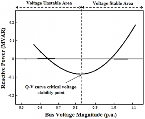
Figure 1. Q-V curve method
The Q-V curve method has several advantages over other static analysis of voltage stability, especially when the lack of reactive power causes the power system to reach its collapse point. As shown in Figure 1, the voltage stability margin is the Megawar distance from zero injection point to below the Q-V curve.
According to Figure 1, an increase in reactive power Q in a stable voltage system will increase the bus voltage. For an instable voltage system, an increase in reactive power Q leads to a decrease in the bus voltage [11-15].
Two new iterative methods are proposed to determine the wind farms maximum size in an interconnected power system. The main difference between these two methods is the incremental trend used to increase the output of new wind farms at the end of each iterative stage and also to consider the effect of increasing the wind power injections on VSMs.
Both methods use hourly peak loads, various hourly loads, and maximum wind farm output power as inputs for the base load flow case. The modified base load flow steps for the first and second methods have been presented below.
Step 1: Determining new wind power injection sites and wind turbine types (DFIG, SCIG or DDSG).
Step 2: Determining the terminal voltage where the wind power injection site will be connected to the network.
Step 3: Determining the power factor at the internal connection point for every new wind power injection site.
Step 4: Determining the seasonal base load flow case to use in the analysis, then calculating VSMs under the worst contingency conditions.
Step 5: Modeling and connecting all new wind farms to the power system at their proposed connection point.
Step 6: Setting all new wind points at zero megawatts with their corresponding MVOR (QOUT).
Step 7: Solving the new base load flow case by modeling new wind farms. Investigating whether the new base load flow case has stable voltage under normal operating conditions or potential events. For this, a possible analysis is used.
Step 8: Determining the power increase step (ΔP) in terms of megawatts, which will increase the output of new wind farms.
5.1 First method: Increasing the output power of new wind farms simultaneously
In this method, the output power of all new wind farms is increased simultaneously at the end of each iteration by ΔP to make voltage instable, or drop the voltage of each shin below a predetermined value (0.9 per unit). The steps of this method have been listed below.
Step 1: Starting with a stable voltage of the new base load flow case obtained from the previous steps.
Step 2: Listing all hourly peak loads in 24 different groups, each group containing one daily hour. Each group contains the maximum system peak loads with a combined load model (ZIP), that occurs in that time for all days of the studied period, because it results in the worst VSM values.
Step 3: Determining the daily hours of the studied season (from 1 to 24) starting at 1 o'clock.
Step 4: Calculating the size of the new wind farms by increasing the total output of all farms by ΔP. Setting the new output power of each wind farm equal to P0 + ΔP.
Step 5: Performing Q-V analysis to calculate the voltage stability margin at the weakest point in the power system and then performing a possible power flow analysis to check the voltage stability.
Step 6: If the VSM is the weakest bus with a stable voltage, then steps 4 and 5 are repeated; otherwise, we go to step 7.
Step 7: Power system voltage instability. The maximum size of each new wind farm is equal to the maximum size obtained before the last iteration which the power system voltage-instability has been reached.
Step 8: Repeat Steps 4 through 7 for all the remaining daily hours of the studied season; from 2 o’clock to 24 o’clock.
Step 9: Finish.
5.2 Second method: Increase the output power of new wind farms independently
The second method calculates the new wind farms maximum size by increasing the output power of each farm independently to reach the voltage stability threshold. At each stage, the size of every one of the wind farms increases by ΔP, and the effect of increasing the output power of each farm on the VSMs is compared. At the end of each iterative step, the output power of a wind farm (wind farm that produces the least negative effect on the VSMs) increases by ΔP, while the size of the other field farms remains constant at its maximum size. The measured values at the end of each iteration will be used in the next iterative step as an initial value. Repeat steps until the increase in the size of a new wind farm results in voltage instability (voltage drop below 9/0 per unit).
The steps are as follows:
Step 1: Starting with a new stable voltage of load flow obtained in the previous steps.
Step 2: Listing all hourly peak loads in 24 different groups, each group containing one daily hour. Each group contains the maximum system peak loads with a combined load model (ZIP), that occurs in that time for all days of the studied period.
Step 3: Determining the daily hours of the studied period (from 1 to 24) starting at 1 o'clock.
Step 4: Starting the iterative steps by increasing the output power of a new wind farm by ΔP, while the output power of the other wind farms remains at their maximum output.
Step 5: Performing a potential power flow analysis to calculate the stability. If the system has stable voltage, we go to step 6 and otherwise we go to step 11.
Step 6: Performing a Q-V curve analysis to calculate and record the lowest VSM (VSM at the lowest point in the power system.)
Step 7: Step 4 and 6 are iterated for all other new wind farms by increasing their output power by ΔP (in megawatt).
Step 8: Comparing VSMs obtained by increasing the output of each wind farm.
Step 9: Increasing the size of the wind farm, which results in the highest VSM (wind farm which has the lowest effect on the VSM). All other wind farms remain at their previous size.
Step 10: Repeating steps 4 through 9 to make the voltage instable on one of the buses.
Step 11: Power system voltage instability. The maximum size of each new wind farm is equal to the maximum size obtained before the last iteration which the power system voltage-instability has been reached.
Step 12: Repeat steps 4 to 11 for all remaining daily hours from 2 to 24.
Step 13: Finish.
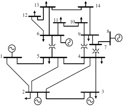
The proposed methods to determine the maximum sizes of two wind farms in the IEEE 14-bus power system have been applied. The one-line version of this system is shown in Figure 2, as well, the data of this network is presented in the ref. [16]. Two new wind farms are in two wider districts with similar wind patterns in buses 7 and 9. DFIG generators in the wind farms were connected at two points of the network at a voltage of 13.8 kV. VSM calculations were performed using a base load flow model that is modified to integrate new wind farms. In the base model, all types of loads are considered as combined power loads (ZIPs).
Figure 2. Single-Line Diagram of IEEE 14-Bus System
Table 1. Types and Characteristics of the Load for Consumption Peak Conditions (Hours 1 to 15 and Hours 21 to 24)
|
Load type Hours 1 to 15 and 21 to 24 in the studied season |
Percentage of total system load |
Constant power P |
Constant current I |
Constant impedance Z |
|
Residential |
28 |
37 |
20 |
43 |
|
Industrial |
45 |
90 |
5 |
5 |
|
Agriculture |
11 |
43 |
20 |
37 |
|
Commercial |
16 |
80 |
10 |
10 |
Table 2. Types and Characteristics of the Load for Consumption Peak Conditions in Summer (Hours 16 to 20)
|
Load type Hours 16 to 20 in the studied season |
Percentage of total system load |
Constant power P |
Constant current I |
Constant impedance Z |
|
Residential |
32 |
37 |
20 |
43 |
|
Industrial |
28 |
90 |
5 |
5 |
|
Agriculture |
15 |
43 |
20 |
37 |
|
Commercial |
25 |
80 |
10 |
10 |
Tables 1 and 2 represent the types of loads as a percentage of total loads, as well combined load in the IEEE 14-bus power system which includes residential, industrial, agricultural and commercial components.
The NEPLAN software, version 5.3.51 was used to analyze the load flow and to create Q-V curves for computing VSMs of the system [17].
Since the greatest limiting factor is for maximizing the size of the field farms under heavy loading conditions, an hourly approach has been used to determine the maximum size of field farms for every hour of the day. Only the daily hours with the highest load level are required to compute the voltage stability margin of system power, because it results in the lowest VSM values. Also, the worst event for VSMs is when the transmission line 13.8 kV is out of service between buses 9 and 14 because it has the lowest voltage stability margin. This case is shown in Table 3. All the calculations presented in this paper are based on this event.
Table 3. Determining the worst contingency
|
Case |
Contingency |
Voltage stability margin (MVAR) |
|
Base Case |
--- |
62.1 |
|
Case 1 |
Open line 3 to 4 |
59.64 |
|
Case 2 |
Open line 4 to 5 |
58.19 |
|
Case 3 |
Open line 2 to 5 |
56.18 |
|
Case 4 |
Open line 10 to 11 |
55.88 |
|
Case 5 |
Open line 2 to 4 |
53.68 |
|
Case 6 |
Open line 12 to 13 |
51.35 |
|
Case 7 |
Open line 2 to 3 |
50.57 |
|
Case 8 |
Open line 1 to 5 |
44.17 |
|
Case 9 |
Open line 6 to 13 |
43.36 |
|
Case 10 |
Open line 6 to 12 |
42.27 |
|
Case 11 |
Open line 6 to 11 |
41.77 |
|
Case 12 |
Open line 13 to 14 |
40.94 |
|
Case 13 |
Open line 9 to 10 |
33.58 |
|
Case 14 |
Open line 9 to 14 |
28.37 |
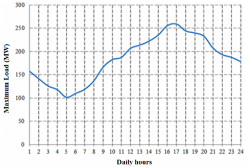
As shown in Figure 3, it is assumed that in the studied chapter, the peak load of the IEEE 14-bus power system occurs afternoon (16-18pm). As expected, the heavy loading conditions during the afternoon leads to the lowest VSMs. This is clearly seen in Table 4 and Figure 4.
Figure 3. Hourly peak load in the studied chapter in terms of MW
Table 4. Hourly peak load in the studied chapter in terms of MW and hourly VSM in terms of MVAR before the wind injection
|
Daily hours for the peak month in the study season |
Maximum hourly peak load (MW) |
The worst calculated VSMs for the worst contingency without wind injection (MVAR) |
|
1 (12am – 1am) |
157.26 |
37.7 |
|
2 (1 am – 2 am) |
141.34 |
38.74 |
|
3 (2 am – 3am ) |
126.15 |
39.97 |
|
4 (3 am – 4am) |
118.03 |
40.62 |
|
5 (4 am – 5am) |
101.74 |
41.91 |
|
6 (5 am – 6 am) |
109.89 |
41.26 |
|
7 (6 am – 7 am) |
119.01 |
40.54 |
|
8 (7 am – 8am) |
137.15 |
39.08 |
|
9 (8 am – 9 am) |
166.42 |
36.97 |
|
10 (9am – 10am) |
182.6 |
35.61 |
|
11 (10am – 11am) |
187.56 |
35.16 |
|
12 (11 am – 12am) |
207 |
33.4 |
|
13 (12 am – 1am) |
213.76 |
32.78 |
|
14 (1 am – 2am) |
222.4 |
31.97 |
|
15 (2 am – 3am) |
235.28 |
30.62 |
|
16 (3 am – 4 am) |
255.65 |
28.45 |
|
17 (4 am – 5 am) |
259.29 |
28.37 |
|
18 (5 am – 6 am) |
244.39 |
29.65 |
|
19 (6 am – 7am) |
240 |
30.09 |
|
20 (7 am – 8am) |
232.83 |
30.86 |
|
21 (8 am – 9am) |
207 |
33.4 |
|
22 (9 am – 10am) |
193.41 |
34.65 |
|
23 (10 am – 11am) |
187.56 |
35.61 |
|
24 (11 am – 12am) |
178.43 |
35.96 |
Figure 4. The lowest hourly VSM in terms of MVAR
The results are presented in Tables 5 and 6 using the first and second methods to determine the maximum wind farm size for each hour in the studied season. In the first method, the size of both wind farms in 30-megawatt steps increases to an instability point. Then, to reach the maximum accurate sizes, the voltages dropped iteratively in the 5-megawatt steps to achieve a stable solution. Applying the first method to determine the wind farms maximum size leads to equal sizes for both farms, which is due to the simultaneous increase in all wind farms size during each iterative step.
The second method results in different maximum sizes for each new wind farm per daily hour. During each iterative step, the size of each wind farm is increased at 30 megawatt steps while its effect on VSMs is observed. At the end of each iteration, the wind farm which has the least negative effect on the VSMs is selected and its size increases to ΔP.
Table 5. Maximum wind power penetration in terms of MW for every daily hour in studied chapter using the first method
|
Daily hours |
Maximum hourly load (MW) |
Injection power in any wind farm (MW) |
Total wind injection (MW) |
VSMs calculated after wind injection (MVAR) |
|
|
Farm 1 (Bus 7) |
Farm 2 (Bus 9) |
||||
|
1 |
157.26 |
115 |
115 |
230 |
25.11 |
|
2 |
141.34 |
115 |
115 |
230 |
22.33 |
|
3 |
126.15 |
115 |
115 |
230 |
24.15 |
|
4 |
118.03 |
120 |
120 |
240 |
20.08 |
|
5 |
101.74 |
120 |
120 |
240 |
22.36 |
|
6 |
109.89 |
120 |
120 |
240 |
21.29 |
|
7 |
119.01 |
120 |
120 |
240 |
19.91 |
|
8 |
137.15 |
115 |
115 |
230 |
22.85 |
|
9 |
166.42 |
115 |
115 |
230 |
24.11 |
|
10 |
182.6 |
110 |
110 |
220 |
24.46 |
|
11 |
187.56 |
110 |
110 |
220 |
23.88 |
|
12 |
207 |
110 |
110 |
220 |
21.62 |
|
13 |
213.76 |
105 |
105 |
210 |
22.66 |
|
14 |
222.4 |
105 |
105 |
210 |
21.65 |
|
15 |
235.28 |
105 |
105 |
210 |
20.3 |
|
16 |
255.65 |
95 |
95 |
190 |
21.08 |
|
17 |
259.29 |
95 |
95 |
190 |
21.03 |
|
18 |
244.39 |
100 |
100 |
200 |
20.91 |
|
19 |
240 |
100 |
100 |
200 |
21.34 |
|
20 |
232.83 |
105 |
105 |
210 |
20.54 |
|
21 |
207 |
110 |
110 |
220 |
21.62 |
|
22 |
193.41 |
110 |
110 |
220 |
23.33 |
|
23 |
187.56 |
110 |
110 |
220 |
23.88 |
|
24 |
178.43 |
110 |
110 |
220 |
24.92 |
This process is iterated to reach the collapse point. Then, in order to obtain the maximum accurate size, the maximum obtained sizes at the last iteration, which resulted in a stable solution, have been increased in 5-megawatt steps to drop the voltage below 0.9 per unit in one of the system buses. Due to space limits, only the second method for the heaviest loading hour (17:00 (4-5 pm)) has been shown in Table 7.
The results of both methods show that the maximum size of the wind farm depends on the used method. The second method allows the injection of larger amounts of wind power in areas where the power system is strong. This results in higher wind power penetration level in most daily hours in studied season than the first method, which does not consider their relative effect on VSMs.
At low wind power penetration level, VSMs are not significantly affected by adding a small amount of wind production, so the reactive power available to existing generators supports wind resources. However, as can be seen in Iteration No. 4 and above, in Table 7, when wind penetration increases significantly, VSMs decrease for any increase in wind farm size, which is due to the reduction in system reactive power.
According to the results, the decrease in VSMs depends on the location and the size of the new wind farms. The bus 7 is better place than bus 9 to extra wind injection. The results of analysis show that determining the size of new wind farms based on the second method allows for maximum use of VSMs and results in a better reduction in VSMs after any incremental increase in wind farm sizes.
Table 6. Maximum wind power penetration in terms of MW for every daily hour in studied chapter using the second method
|
Daily hours |
Maximum hourly load (MW) |
Injection power in any wind farm (MW) |
Total wind injection (MW) |
VSMs calculated after wind injection (MVAR) |
|
|
Farm 1 (Bus 7) |
Farm 2 (Bus 9) |
||||
|
1 |
157.26 |
150 |
85 |
235 |
24.05 |
|
2 |
141.34 |
140 |
95 |
235 |
25.91 |
|
3 |
126.15 |
150 |
90 |
240 |
18.87 |
|
4 |
118.03 |
150 |
90 |
240 |
20.27 |
|
5 |
101.74 |
150 |
95 |
245 |
19.03 |
|
6 |
109.89 |
150 |
90 |
240 |
21.58 |
|
7 |
119.01 |
150 |
90 |
240 |
20.09 |
|
8 |
137.15 |
135 |
100 |
235 |
20.78 |
|
9 |
166.42 |
140 |
90 |
230 |
24.4 |
|
10 |
182.6 |
135 |
90 |
225 |
23.7 |
|
11 |
187.56 |
135 |
90 |
225 |
23.1 |
|
12 |
207 |
130 |
90 |
220 |
21.84 |
|
13 |
213.76 |
130 |
90 |
220 |
21.02 |
|
14 |
222.4 |
125 |
90 |
215 |
20.95 |
|
15 |
235.28 |
120 |
90 |
210 |
20.46 |
|
16 |
255.65 |
120 |
80 |
200 |
19.91 |
|
17 |
259.29 |
120 |
80 |
200 |
19.85 |
|
18 |
244.39 |
125 |
80 |
205 |
20.33 |
|
19 |
240 |
120 |
90 |
210 |
19.93 |
|
20 |
232.83 |
125 |
90 |
215 |
19.81 |
|
21 |
207 |
130 |
90 |
220 |
21.84 |
|
22 |
193.41 |
135 |
90 |
225 |
22.42 |
|
23 |
187.56 |
135 |
90 |
225 |
23.1 |
|
24 |
178.43 |
135 |
95 |
230 |
23 |
Table 7. Iterative steps to calculate the maximum wind farm size using the second method for daily hour 17
|
Repeat number |
Farm 1 in Bus 7 |
Farm 2 in Bus 9 |
The lowest voltage stability margin (MVAR) |
Description |
|
Maximum wind farm size (MW) |
||||
|
Base Case |
0 |
0 |
28.37 |
No wind injection |
|
Repetition 1 |
30 |
0 |
28.46 |
Increase farm 1 |
|
|
0 |
30 |
28.38 |
Increase farm 2 |
|
Result 1 |
30 |
0 |
28.46 |
Setting farm 1 at 30 MW |
|
Repetition 2 |
60 |
0 |
28.16 |
Increase farm 1 |
|
|
30 |
30 |
28.15 |
Increase farm 2 |
|
Result 2 |
60 |
0 |
28.16 |
Setting farm 1 at 60 MW |
|
….. |
….. |
….. |
….. |
….. |
|
Result 6 |
120 |
60 |
22.26 |
Setting farm 1 at 120 MW |
|
Repetition 7 |
150 |
60 |
Unstable |
Increase farm 1 |
|
|
120 |
90 |
Unstable |
Increase farm 2 |
|
Result 7 |
Increase the size obtained by repeating 6 in steps of 5 MW |
|||
|
Repetition 8 |
125 |
60 |
21.72 |
Increase farm 1 |
|
|
120 |
65 |
21.74 |
Increase farm 2 |
|
Result 8 |
120 |
65 |
21.74 |
Setting farm 2 at 65 MW |
|
….. |
….. |
….. |
….. |
….. |
|
Repetition 11 |
125 |
75 |
19.84 |
Increase farm 1 |
|
|
120 |
80 |
19.85 |
Increase farm 2 |
|
Result 11 |
120 |
80 |
19.85 |
Setting farm 2 at 80 MW |
|
Repetition 12 |
125 |
80 |
Unstable |
Increase farm 1 |
|
|
120 |
85 |
Unstable |
Increase farm 2 |
|
Total injectable wind power |
200 MW |
|
||
In this paper, two methods have been provided to determine the new wind farms maximum size which can be injected in power systems without reaching voltage instability. The reliance on a voltage stability-based approach to determine the maximum wind farm size can limit the integration of wind power in the future due to the decrease in the voltage stability margin in other parts of the power system.
In order to maximize the influence of wind on power systems, the new wind farms maximum sizes should be determined using the second method. The second method leads to more wind power penetration than the first method in most daily hours. In the methods provided, accurate wind speed data in new wind penetration sites are not required, but only the heaviest loading hours are required with load type specification (percentage of CI, CP, and CZ) to determine the wind farms maximum size in all daily hours.
The new methods proposed in this paper provide wind farm developers and electric company planners a tool to determine the wind farms maximum size which are safe regarding voltage stability. These new methods can be applied to any number of wind farms and in every power system.
[1] Linh, N.T. (2009). Voltage stability analysis of grids connected wind generators. 2009 4th IEEE Conference on Industrial Electronics and Applications, pp. 2657-2660. https://doi.org/10.1109/ICIEA.2009.5138689
[2] Coath, G., Al-Dabbagh, M. (2005). Effect of steady state wind turbine generator models on power flow convergence and voltage stability limit. Available at https://citeseerx.ist.psu.edu/viewdoc/download?doi=10.1.1.492.6005&rep=rep1&type=pdf.
[3] Chinchilla, M., Arnalte, S., Burgos, J.C., Rodrigues, J.L. (2006). Power limits of grid-connected modern wind energy systems. Renewable Energy, 31(9): 1455-1470. https://doi.org/10.1016/j.renene.2004.03.021
[4] Pal, M.K. (1993). Voltage stability: Analysis needs, modeling requirement and modeling adequacy. IEE Proc. C, 140(4): 279-286. https://doi.org/10.1049/ip-c.1993.0041
[5] Pal, M.K. (1992). Voltage stability conditions considering load characteristics. IEEE Trans., PWRS, 7(1): 243-249. https://doi.org/10.1109/59.141710
[6] Li, Y.H., Chiang, H.D., Li, H., Chen, Y.T., Huang, D.H., Lauby, M.G. (2006). Power system load ranking for voltage stability analysis. IEEE Trans., 8. https://doi.org/10.1109/PES.2006.1709345
[7] Taylor, C.W. (1997). Maybe I can’t Define Stability, but I know it when I See it. Presented at IEEE/PES panel on Stability Terms and Definitions, New York, February, 1997.
[8] EPRI Project 849-7 Final Report EL-5003, “Load Modeling for Power Flow and Transient Stability Computer Studies”, January 1987.
[9] Price, W.W., Wirgau, K.A., Murdoch, A., Mitsche, J.V., Vaahedi, E., El-Kady, M. (1988). Load modeling for power flow and transient stability computer studies. Power Systems, IEEE Transactions on Power Systems, 3(1): 180-187. https://doi.org/10.1109/59.43196
[10] Taylor, C.W. (1994). Power System Voltage Stability. 1994 by McGraw-Hill, Inc. page 72.
[11] Kundur, P. (1994). Power System Stability and Control, New York: McGraw- Hill.
[12] Nakhi, P.R., Kamarposhti, M.A. (2020). Multi objective design of type II fuzzy based power system stabilizer for power system with wind farm turbine considering uncertainty. Int. Trans. Electr. Energy Syst, 30(4): e12285. https://doi.org/10.1002/2050-7038.12285
[13] Eslami, M., Kamarposhti, A. (2019). Optimal design of solar–wind hybrid system connected to the network with cost-saving approach and improved network reliability index. SN Appl. Sci., 1(12): 1-12. https://doi.org/10.1007/s42452-019-1710-y
[14] Kamarposhti, M.A., Mozafari, S.B., Soleymani, S., Hosseini, S.M. (2015). Improving the wind penetration level of the power systems connected to doubly fed induction generator wind farms considering voltage stability constraints. J. Renewable Sustainable Energy, 7: 043121. https://doi.org/10.1063/1.4927008
[15] Kamarposhti, M.A., Soodabeh, S., Seyed Babak, M., Hosseini, Mehdi, S. (2015). An approach to optimal location of SVC in power system connected to DFIG wind farms based on maximization of voltage stability and system loadability. J. Intell. Fuzzy System, 29(5): 2147-2157. https://doi.org/10.3233/IFS-151690
[16] Kodsi, S.K.M., Cannizares, C.A. (2003). Modeling and simulation of IEEE 14-bus system with FACTS controllers. Technical Report 2003-3, University of Waterloo, Waterloo, Ontario, Canada.
[17] "Neplan - Planning and Optimization System for Electrical Networks", Busarello+Cott+Partner Inc. (BCP), www.neplan.ch (current 29 July 2003).