Relangi Naga Durga Satya Siva Kiran* | Chaparala Aparna | Sajja Radhika
© 2021 IIETA. This article is published by IIETA and is licensed under the CC BY 4.0 license (http://creativecommons.org/licenses/by/4.0/).
OPEN ACCESS
Groundwater quality assessment is primarily intended to determine whether the water in a particular area can be used for aquatic purpose or not. The assessment comprises analysis of physical, chemical and microbiological characteristics of groundwater samples. The quality of groundwater can be evaluated through few standard conventional methods viz. Water Quality Index, Canadian Council of Ministries Environmental Water Quality Index and Weighted Arithmetic Water Quality Index etc. In addition to the conventional methods, multivariate statistical methods like Principal Component Analysis, Factor Analysis and Cluster Analysis can also be used to assess the groundwater quality. As these methods are descriptive models, they are inadequate to predict the quality of unknown groundwater sample. Hence, an efficient predictive model is desirable to analyze the characteristic parameters of groundwater samples and predict the quality of an unknown sample. The sample may have both crisp and fuzzy values. Conventional supervised learning methods may not be suitable for constructing the required prediction model as they are not suitable for handling fuzzy input data. Therefore, simplified fuzzy adaptive resonance theory model is an appropriate choice for accomplishing the task of building the prediction model. The present work proposes to assess the quality of groundwater by applying the Weighted Arithmetic Water Quality Index method and Simplified Fuzzy Adaptive Resonance Theory model by considering 7 groundwater quality parameters. The accuracy of afore mentioned approach seems to be pleasing when compared to counter parts like Back propagation and Random Forests classifiers.
adaptive resonance theory, artificial neural networks, back propagation, fuzzy water quality index, random forests, simplified fuzzy ARTMAP, weighted arithmetic water quality index
Water is the prime resource of all living beings. The primary responsibility of the groundwater monitoring networks or water supply systems is to evaluate the quality of the groundwater by using physical, chemical and biochemical parameters. The groundwater quality parameter values are always continuous in nature. The best example of groundwater monitoring system is rural water supply and sanitation systems. The officials at these stations have to collect the groundwater samples with chemical and microbiological parameters like pH, Coli form and fecal coli form etc. from different locations in their assigned premises at regular intervals and get the values of the parameters to assess the quality of the groundwater.
The groundwater pollution is one of the environmental problems and it is caused by various factors like discharge of agricultural wastage, runoff produced from pharmaceutical industries, paints and oil manufacturers well as other industries also. In many places, the groundwater is directly used by the human beings for their living purposes but the consumption of groundwater directly without any water treatment will show adverse effect on health of the human beings. So to rid of this defect, fresh water from the groundwater must be processed. To do this, we need to identify the polluting sources those dilute the quality of the groundwater.
In this research work, an attempt has been made to evaluate the ground water quality class label of unknown data sample and groundwater classification based on its purity. To this end we used two ANN models viz., Back propagation, Random Forests and one Neuro Fuzzy Model called Simplified Fuzzy Adaptive Resonance Theory model. After implementing these models, we made comparative study of these three models to find out the best model to assign the groundwater quality class label of the given unknown data sample. In this process, first we have to evaluate the grade of the groundwater sample by using WAWQI method of each sample in the data set. Then provide the data set as input to train the three models considered in this work. After finishing the training process the learned models can be used to assess the class label of the given unknown groundwater sample.
The Studies on the groundwater quality is categorized into four types i.e., conventional methods, multivariate statistical methods, artificial neural networks and fuzzy logic algorithms for obtaining groundwater quality evaluation and grade assignment.
Firstly, regarding conventional methods category, i.e., conventional groundwater quality assessment methods were studied. Groundwater is used for drinking and other living purposes directly in some areas and at the same time it is polluted by the unethical activities by human beings and heavy usage of groundwater also lead to groundwater contamination. Therefore, evaluation of groundwater quality is highly recommended. By using the conventional methods one can easily calculate the groundwater quality. The quality value produced by the conventional methods are easily understood by the layman. The conventional methods are used to evaluate both the ground and surface water quality. The problems associated with the conventional methods are: there is no universal standard in selecting the number of parameters to evaluate the quality of the groundwater and based on the experts knowledge the parameters are assigned with different weights in the evaluation process which influence the quality of the groundwater.
The term water quality index is first coined by Horton in 1965. The WQI is first developed by Horton [1] by considering 10 water quality parameters to evaluate the quality of the water in United States. Horton is first person who converted the complex water quality parameter values into a single index number and can be easily understood by the general public. Brown et al. [2] proposed an enhanced water quality index by adding 2 more important water quality evaluation parameters to Hortons method viz. temperature and obvious pollution to the Horton WQI method. Cude [3] developed Oregon Water Quality Index (OWQI) in 1970 for evaluate the streams and this method is discontinued in 1983 due to excessive resources needed to calculate and report the water quality index value.
The researchers Khwaja Anwar et al. [4] assessed the groundwater quality at Aligarh City, India, by applying WQI method. Collected total of 80 groundwater samples from 40 sampling locations during 2 seasons pre monsoon and post monsoon seasons respectively. All these samples are subjected to 14 physical and chemical parameters. These physical and chemical water quality parameters gathered are analysed according to the guidelines issued by Bureau of Indian Standards under Indian Standard Drinking Water Specification IS:10500:2012 [5], the groundwater quality of each data sample is evaluated by using the WQI method. This study reveals that 4 locations during the pre-monsoon and 5 locations during post monsoon season exhibited excellent water quality and directly used for human consumption. The groundwater quality in the rest of the sampling locations belongs to the category either good or moderately contaminated. This work also found that pH, Alkalinity, Magnesium, Hardness, Fe, Calcium and TDS are the parameters lead to groundwater contamination. Gupta et al. [6] performed comparative analysis of 5 water quality evaluation methods to classify the costal water quality by considering 6 water quality parameters. Applied the 5 water quality indices to determine which one is the best method. This comparative study reveals that the multiplicative method to evaluate the water quality is the best suitable method to classify the water samples from the study area. Zotou et al. [7] performed comparative analysis of 7 water quality indices to evaluate the water quality of Mediterranean River. This study reports that CCME water quality index is most efficient index among the other water quality indices considered in this work. CCME WQI is also a powerful tool to evaluate the quality of any kind of water i.e. surface water or groundwater. Uddin et al. [8] assess the quality of the groundwater by applying the CCME water quality index method. Collected groundwater samples from 17 sampling locations during January 2017. The sampling locations belongs to Nuclear Power Plant area, Pabna District, Bangladesh. All the groundwater samples are analysed for 22 physical and chemical parameters. By applying the CCME method it was observed that the groundwater from the study area is not suitable for drinking purpose.
Saleem et al. [9] have collected groundwater samples with 9 physical and chemical parameters from 10 sampling locations of Grater Noida region located in Uttar Pradesh State, India. These samples are analysed using by WQI method and found that most of the samples are having good groundwater quality and the authors also suggested that some treatment is needed before using it. Rajendran et al. [10] have investigated the groundwater quality of Turuchurapalli city located in Tamil Nadu State, India. To assess the data analysis they have collected samples with 19 physical and chemical parameters from 10 sampling locations during March to August 2015. The preliminary data analysis states that all the physical and chemical parameters exceeded its limits and heavy metals in the study are below the prescribed limits if it continues that the groundwater at the considered sampling sites is not suitable for potable purpose. The samples from the study area are contaminated due to leakages from underground fuel tanks and septic tanks, seepage through landfills, pesticides used in farms. Asadi et al. [11] utilized WQI and Irrigation Water Quality Index used locate the suitable area of water pumping for drinking and agricultural purposes in the Tabriz aquifer, located in East Azerbaijan province, northwest Iran. Collected 39 samples with 12 physical and chemical parameters during 2003 to 2014. This study reports that groundwater from the most of the sampling locations is good for human consumption. About 37% of the groundwater is highly suitable for irrigation purposes and 73% of the groundwater is moderately suitable for irrigation purposes.
Verma et al. [12] assessed the suitability of groundwater for potable purpose by the human beings by considering groundwater samples with twelve physical and chemical parameters that are T-hard, TDS, pH, calcium and Magnesium etc., collected during two seasons pre monsoon and post monsoon in the year 2014-2015 from Bokaro district, Jharkhand State, India. The Geographic information system based on water quality index model implemented to ascertain the groundwater quality. The analysis depicts that the groundwater quality is degraded in monsoon season by decreasing the concentration of the considered 5 parameters. This work concludes that groundwater is not suitable for drinking purpose in both seasons and also finds that groundwater is degraded due to anthropogenic activities. Recently a modified water quality index is proposed by Shankar and Raman et al. [13] called as Modified Water Quality Index (MWQI) based on CCME by assigning the relative weights to the important groundwater quality parameters and applied it for evaluating the groundwater quality of Bommanahalli area in Bangalore. Collected groundwater samples from 11 sampling locations about 10 parameters during pre monsoon and post monsoon seasons 2018. They reported that the about 93.33% of groundwater is exhibits poor water condition and the groundwater from the sampling locations is not suitable for drinking purpose.
The second category is the Multivariate statistical category. In this study, we reviewed the applicability of multivariate statistical methods to evaluate and classify the groundwater data. Multivariate statistical methods are the integration of the various statistical models intended to find the hidden and implicit patterns in the data by considering more than one variable in the data. Multivariate analysis can be applied when the given data set possess some characteristics that are large volumes of data with huge number of dimensions, data is dynamic, correlations among the data are very difficult to assess, etc. Some popular multivariate statistical methods like Multilinear Regression, Principal Component Analysis, Cluster Analysis and Factor Analysis are often applied to assess the groundwater quality. Krishna et al. [14] applied multivariate statistical techniques viz. Factor Analysis and PCA to assess the metal pollution and to find the impact of trace elements in surface and groundwater at Patancheru industrial area near Hyderabad City, India, and a number of chemical and pharmaceutical industries are located nearer to the study area. Wastage produced by these industries are directly discharged into surrounding lands, irrigation fields and surface bodies forming point and non-point of contamination for groundwater. The authors first applied PCA and identified four factors which deteriorated the surface water. Factor1 reveal that arsenic contamination in surface area comes mainly from paint, pharmaceutical, fertilizers and pesticides industries. Factor2 reveal that the surface is deteriorated by anthropogenic activities. Factor3 reveal that surface water deteriorated due to agricultural activities, Factor4 reveals that geogenic process led to surface water deterioration. Gulgundi et al. [15] utilized multivariate statistical techniques PCA and APCS-MLS for evaluating the groundwater quality and to know the sources those decrease the groundwater quality. To the end collected 68 samples and were analysed for 14 physicochemical parameters. The collection of samples was done during pre monsoon and post monsoon seasons. The statistical data analysis states that concentration values of physiochemical parameters exceed its prescribed limits during post monsoon season when compared with pre monsoon season. This work reports that the groundwater from the study area is not suitable for drinking purpose. The sources which lead to groundwater contamination are septic tank sewage, bedrocks, waste materials from manufacturing industries and also by geogenic activities. There are some unidentified factors which also degrade the groundwater quality.
The third category is Neural Networks. The ANN is a branch of Artificial Neural Networks. The ANN models are used in various domains like Finance, Health Care, Business, Telecommunications etc. The ANN algorithms are used in the field of water quality evaluation and classification. The ANN models are well suited for classify or cluster the groundwater samples into classes or clusters. The ANN model is a non linear modeling method based on the input variables also termed as independent variables to find the values of one or more variables these variables are also called as dependent variables. In this category, we review the applicability of neural networks and different neural network constructions to classify and predict groundwater quality. With these types of networks one can build a groundwater quality classification and prediction model by integrating the physical, chemical or microbiological parameters of the groundwater. These models are used by the groundwater quality monitoring stations to identity the places where groundwater quality is suffering from contamination and also identify the cause which leads to groundwater contamination. The Back propagation model is a frequently applied in groundwater purity and grade assessment and prediction [16-18]. This study evaluates the utility of BPNN, Random Forests and SFART neural networks for classifying and predict class label means the water quality grade of the groundwater data. Kheradpisheha et al. [19] implemented Back propagation model with five training algorithms to evaluate groundwater quality. The authors collected 260 samples from 13 wells during the period 2003 to 2013 with 18 parameters from Bahabad plain area located in Central Province of Iran. This work resulted in assessment of SO4, EC, NO3 and CL parameter values are more accurate. Purkait et al. [20] examined the impact of arsenic contamination in groundwater by Back propagation neural network model and compared the accuracy with Multi Linear Regression and Active Set Support Vector Regression models. To carry out this work 85 groundwater samples with parameters like pH, Sp. Cond, TDS, Salinity, DO, Depth of the tube well and Eh are collected from different locations of Malada district, West Bengal, India. This model consists of the above stated 7 geological groundwater quality parameters as input and one output node to assess the impact of arsenic on groundwater quality. The configuration of this model consists of four layers and one input layer with 7 neurons, two hidden layers with 15 neurons and the output layer with a single neuron. This work reports that the Back propagation model exhibits higher accuracy to assess the arsenic contamination in groundwater compared with the other considered models. Ganga Devi [21] applied Random Forests model for predicting the groundwater quality class label and to check the groundwater from the study area is suitable for drinking purpose or not. Wang et al. [22] proposed an enhanced random forest model for short term prediction groundwater level of Daguhe River groundwater source field, in Qingdao, China.
The fourth and last category is the Neuro-fuzzy systems. We reviewed the usage and construction of Neuro-Fuzzy systems to assess the groundwater quality. The Adaptive Neuro-Fuzzy system is the combination of ANN and fuzzy inference systems.
Mohammad et al. [23] developed fuzzy water quality index (FWQI)method to overcome the problems involved in assessing the water quality by conventional water quality index methods like identifying the water quality parameters and assigning the relative weight of the groundwater quality parameters etc. FWQI was developed based on Mamdani fuzzy inference system. A total of 7 fuzzy water quality index methods with different water quality parameters haven been developed based on trapezoidal and triangular fuzzy membership functions. The FWQI method performs better than the conventional methods in assessing the groundwater quality. Nasr et al. [24] developed a model called FWQI to assess the groundwater suitability for the potable purpose and the area under study is Yazd province located in the Centre of Iran. From this area there is a huge withdrawal and usage of groundwater which directly influenced the groundwater level and hence chances to decrease the groundwater quality are high. So it is important to handle this situation, by collecting data samples with 12 physical and chemical parameters including TH, TDS, T-Alk, Pb, Cd, etc. from 71 sampling locations and are analyzed using fuzzy water quality index method to check the quality of the groundwater for potable purpose. This work reveals that there is a difference in the groundwater quality grades assignment between the conventional and the FWQI method. The FWQI method proposed by the authors, is well suited to assign groundwater quality grades. This work finally states that few of the samples belong to excellent quality, more than 50 percent of the samples belong to good water quality and 13 samples belongs to poor water quality. Sahu et al. [25] have done a comprehensive study regarding groundwater quality of wells in the urban area of Sundergarh district, Odisha state, India. A huge number of firms are located in the study area viz. coal, iron, manganese etc. The study area is contaminated with the wastage discharged by firms stated above. In addition to these industries, the agricultural practices are also affecting the groundwater quality. To carry out this task the authors have collected data samples from 20 sampling locations during three seasons i.e, summer, rainy and winter seasons during the years 2009-2010. These samples are subjected to 12 groundwater quality parameters and some of them are pH, Hardness, BOD, Do, TDS etc. This work resulted that the groundwater in the study area is suitable for human consumption with quality accuracy. Adaptive Neuro Fuzzy Inference system with a hybrid learning rule found the groundwater quality with reasonable accuracy and states that the groundwater in the study area is suitable for human consumption. Dahiya et al. [26] applied the fuzzy synthetic evaluation method to assess the groundwater quality for drinking purpose. Collected 42 groundwater samples from 15 sampling locations. These samples are analysed for 16 physical and chemical parameters but only 10 groundwater quality parameters are taken into consideration to assess the groundwater quality by the fuzzy synthetic evaluation method. These 10 parameters are divided into 4 groups based on the experts opinion with respected to drinking water quality criteria. Mamdani fuzzy implication method is used to generate the rule base and formed 55 rules. This work reports that the 64% of the groundwater samples are suitable for drinking purpose.
Gharibi et al. [27] developed a novel water quality index based on fuzzy logic for the assessment of surface water quality for drinking purpose. The novel fuzzy water quality index is superior than the conventional water quality assessment models like NSFWQI, CCMEWQI etc.
Kiran Relangi et al. [28] performed comprehensive analysis of various methods like conventional, statistical, neural networks, fuzzy logic inference systems used in both groundwater quality and surface water quality assessment.
From the literature the following points are observed.
•There is no universal method to evaluate the groundwater quality.
•There exist huge number of methods in selecting the groundwater quality parameters and their standards.
•The groundwater level is increased in monsoon season which in turn carries the pollutants to the water table hence the groundwater quality is decreased in monsoon season. It indicates that monsoon is an important factor affecting the groundwater quality.
•The ANN and fuzzy inference models are used for groundwater quality assessment and groundwater quality class label prediction. The conventional and multivariate statistical models are also used in the past studies for groundwater quality grade assessment only.
3.1 Experimental setup
By considering the 3 classifiers viz. Back propagation, Random Forests and Simplified Fuzzy Adaptive Resonance (SFART) experiments are conducted. These experiments are implemented by using Python 3.7.4 programming language. In order to develop these 3 classifiers models Python Programming Integrated Development Environment PyCharm community Edition is used. The development process is done on Core i5-8250U CPU with 1.6 GHz processor, 8 GM RAM running on Windows 10 64-bit operating system. For empirical study, 1020 data samples of groundwater of the year 2019 are collected from Water Quality Monitoring Lab, RWS&S Sub-Division, Narsapuram, West Godavari, Andhra Pradesh, India. The samples consist of 7 physical, chemical and microbiological parameters viz. Potential Hydrogen, Temp, Conductivity, BOD, Fecal Coliform, Total Coliform and Nitrate+Nitrite. For the training and testing of the 3 models the data samples were split into train and test sets with data 70% and 30% respectively. In these classifiers development process sklearn, numpy, pandas and matplotlib libraries were used. The input to these three models is the sampling data with 7 physical, chemical and microbiological parameters. But the samples don’t possess the groundwater quality index or grade to ascertain the index we employed the WAWQI [29] method given in Eq. (2). The groundwater quality is classified into five classes as excellent, good, poor, very poor and not suitable for drinking purpose based on the calculated value using the WAWQI method. The above stated three models takes input parameter values between 0 and 1. To transform the real values into values between 0 to 1 we use min-max normalization technique [30] given in Eq. (1).
The min-max normalization formula is presented below.
$n e w X_{i}=\frac{X i-X m i n}{X \max -X \min }$ (1)
In the above Eq. (1), the parameter xi is the current value to be transformed, xmin and xmax are the smallest and largest values of the feature respectively.
3.2 Evaluation of WQI
A number of indices are existed to assess the purity of both groundwater and surface water they are National Sanitation Foundation Water Quality Index (NSFWQI), Weight Arithmetic Water Quality Index (WAWQI), Canadian Council of Ministries of the Environment Water Quality Index (CCMEWQI), Oregon Water Quality Index (OWQI) etc. Tyagi et al. [31] presented the evaluation of water quality through the conventional assessment methods along with its merits and demerits. The authors also reports that there is no universal method to assess the water quality.
In order to determine the quality grade of each sample we employ the popular Weighted Arithmetic Water Quality Index method and is given in Eq. (2). This method computes the groundwater quality grade with respect to water purity by considering the above stated 7 parameters.
Water Quality Index $=\frac{\sum_{j=1}^{n} Q j W j}{\sum W_{j}}$ (2)
In the above Eq. (2) Wj represents the relative weight of the jth parameter and Qi represents the quality value for jth parameter.
The parameter Qi value is determined using the following Eq. (3).
$Q i=\frac{((V j-V 0) * 100)}{(S j-V 0)}$ (3)
In the above Eq. (3), Vi denotes the value of the ith parameter in analyzed water, V0 is the ideal value of the parameter in pure water. V0=0 (excluding pH=7.0 and DO=14.6 mg/l) and Sjis the recommended standard for jth parameter.
3.3 Back propagation algorithm
Back propagation Neural Network is a supervised learning model [32], and is frequently used in groundwater quality evaluation for assessing the grade of the groundwater or to assess the impact of a single or multiple water quality parameters. In this work we used the Back propagation model to classify groundwater quality grade assignment.
Back propagation model is a collection of layers with computational processing units also termed as neurons which are the elementary units of an ANN model, the elementary units in each layer are connected with the units in the next layer using weights. Generally, there is one input layer and an output layer with a finite number of hidden layers in the Back propagation model. The number of hidden layers explicitly depends on the nature of the problem. The accuracy of the model directly depends on the structure of the model means, the number of neurons in the input and hidden layers, the type of the activation function used to squash the input value within a range and the training method. One popular way to find the optimal structure of the model by using the trial and error method or to use the optimization techniques. There are no predefined thumb rules to decide the optimal structure. We present the input feature vector to the input layer with the 7 parameter values along with the class label. The class label of each sample is obtained by applying the Weighted Arithmetic Water Quality Index method which is given in Eq. (2). The output of the input layer is given as input to the hidden layer and the hidden layer also having 7 neurons after performing the processing at the hidden layer the output of the hidden neurons passed as input to the output layer with a single neuron which represents the groundwater quality grade. After calculating the groundwater quality grade at the output neuron, we proceed in the backward direction by calculating the error of the observed value by measuring the difference between the observed value and true value. Finally, the weights are adjusted between output-hidden layers as well as hidden and input layers to minimize the error between the observed value and true value. To do this we employ the gradient descent as training algorithm. This model achieved best accuracy values after 4000 iterations shown in Table 1.
3.4 Random forests algorithm
The Random Forests is an ensemble classifier algorithm developed by Breiman [33] Professor in Statistical Department, University of California, Berkeley, the origin of this algorithm is decision tree. The working procedure of this algorithm is to construct various decision trees based on random sampling and merge them into a single Random Forests tree and the final decision is made by using majority voting method. Random Forests model with bootstrap random sampling is used in this work to classify groundwater samples. This model is experimented by increasing the number of decision trees. Initially, we choose 5 random trees and then increased the number of trees up to a maximum of 50 trees. This model exhibits 91.30% classification accuracy with 25treesand it gives the same performance even the number of trees is increased to 50. The results obtained by this model are shown in Table 2. From the results it is noticed that by increasing the number of trees the classifier perforce is also increasing.
3.5 Simplified fuzzy ARTMAP algorithm
The concept of fuzzy sets describing imprecision or vagueness and is introduced by Zadeh [34] in 1960s. Fuzzy set theory is also called as theory of uncertainty. Fuzzy adaptive resonance theory is first introduced by Carpenter et al. [35]. The Simplified Fuzzy Adaptive Resonance Theory [36] (Simplified fuzzy ARTMAP) is a hybrid supervised model. This model is an adaptive learning model by adjusting the weights in the weight vector. Adaptive learning means adjusting the parameter values during its operation in a dynamical environment with respect to the features of the input data to find the best fit between the output produced by the model and the actual one. Simplified fuzzy ARTMAP combines the best features from the ANN and fuzzy theory. The main drawback of the ANN is it cannot process data with uncertainty. The bottleneck of the fuzzy theory is that it doesn’t have learning mechanism but can represent and process the data with uncertainty using linguistic terms. Now the best features from these two models are merged into a hybrid system known as neuro-fuzzy systems.
Input the feature vectors to the SFART network. The feature vector consists of the 7 groundwater quality parameter values and the class label i.e. the groundwater quality grade of that particular sample. From the input feature vector, this model first computes the complement coding vector. If it is the first pattern presented as input to the SFART network then the augmented input pattern values form the first weight vector. Apply the activation function with the augmented input pattern. Calculate the match tracking function value with the augmented input pattern and if the match tracking function value is greater than the vigilance parameter then the model said to be in resonance state and its category is same as the weight vector category then update the weight vector to learn from the input pattern else next node is considered for learning process. The above training process is repeated until the termination condition holds. This model shows the best results in groundwater quality grade assessment compared with the BPNN and Random Forests models considered in this work. This model achieves 93.93% classification accuracy score even the number of iterations is increased from 500 to 5000. Hence this model outperforms the other two models used in groundwater quality grade assessment. The details of Simplified FARTMAP model are presented below.
Step 1: The input feature vector is denoted as FV=(ai1,ai2,ai3, ..., aid) of d dimensions and its class category is Ci, initialize the vigilance parameter ρ as 0<ρ<1, set a small value for α and the number of iterations also.
Step 2: Compute the augment of the input feature vector by performing the complement encoding of FV as given below:
$AIFV i=(a i 1, a i 2, a i 3 \ldots \ldots a i d, 1-a i 1,1-a i 2,1$$-a i 3, \ldots .1-$ aid $)$ (4)
Step 3: AIFVi is the first input feature vector in Ci category, then assign the weight vector Wi as AIFVi and go to step 10.
Step 4: If AIFVi is the input feature vector whose class category already present then calculate the activation function of Tj(AIFVi) as given below:
$T j(A I F V i)=\frac{\left\|A I F V i_{\Lambda} W j\right\|}{\alpha+\|W j\|}$ (5)
Step 5: Select the weight node K with the maximum value after applying the activation function which is given below:
$T j($ AIFVi $)=\operatorname{maxTj}($ AIFVi $)$ (6)
Step 6: Calculate the match tracking function MFK(AIFVi) of the node K which gets the maximum activation value, ifMFK> ρ and Ci=CK then only update the weight vector using the following equation and go to Step 10.
$W_{k}^{n e w}=W_{k}^{\text {old }}+\left\|A I F V i_{k} W_{k}^{\text {old }}\right\|$ (7)
Step 7: If MFK> ρ and Ci≠CK then assign ρ to MFK(AIFVi) and increment it by a small value of e as given below:
$\rho=M F K(A I F V i)+\varepsilon$ (8)
Step 8: If MFK<ρ and if some more weight vector nodes exist then consider the next highest winner WK among the other nodes and go to Step 6, Otherwise go to Step 9.
Step 9: Create a new weight vector node W1 and assign W1=AIFVi and assign it class to Ci.
Step 10: If no more feature vectors present go to step 11, else increment i as i¬i+1 and go to Step 1.
Step 11: Terminate the training process if number of iterations are finished.
This subsection presents the comparison of classifier accuracy metrics between the 3 models BPNN, Random Forests and SFART models. We had analysed that the performance of the 3 models BPNN, Random Forests and SFART models for 5000 iterations. The Back propagation, Random Forests and Simplified Fuzzy Adaptive Resonance Theory models are observed with the classifier accuracy metrics. The results are provided in Table 1, Table 2 and Table 3. We first analysed the empirical results of the three models by comparing them with the other models considered in this study. Later we analysed the pros and cons of each model separately.
As presented in Table 1, the classifier accuracy values are presented for BPNN model based on number of iterations. As shown in the Table 1 each classifier is trained for about 500 to 5000 iterations but From Table 1 it is observed that the BPNN model exhibits good prediction rate 93.07% at 4000 iterations only. As presented in Table 2, the classifier accuracy values are presented for Random Forests model based on number iterations and number of decision trees. From the Table 2 it is observed that this model shows good prediction rate at 2500 iterations with 25 number of decision trees and the model exhibits the same prediction rate even the number of iterations and decision tress are increased to 5000 and 50 respectively.
Table 1. BPNN algorithm classifier accuracy metrics values
|
Name of the Metric No of Iterations |
Mean absolute error |
Mean squared error |
Root mean squared error |
Classifier accuracy score |
Precision |
Recall |
f Score |
|
500 |
0.1818 |
0.3896 |
0.6241 |
89.00 |
0.86 |
0.90 |
0.87 |
|
1000 |
0.3636 |
1.246 |
1.116 |
92.20 |
0.81 |
0.88 |
0.84 |
|
1500 |
0.1688 |
0.3766 |
0.6136 |
92.64 |
0.91 |
0.91 |
0.90 |
|
2000 |
0.1558 |
0.2597 |
0.5096 |
92.64 |
0.81 |
0.88 |
0.84 |
|
2500 |
0.3506 |
1.1558 |
1.0751 |
92.20 |
0.81 |
0.88 |
0.84 |
|
3000 |
0.2077 |
0.3896 |
0.6241 |
90.04 |
0.81 |
0.87 |
0.83 |
|
3500 |
0.1818 |
0.3896 |
0.6241 |
92.64 |
0.86 |
0.90 |
0.87 |
|
4000 |
0.1688 |
0.4025 |
0.6345 |
93.07 |
0.87 |
0.91 |
0.89 |
|
4500 |
0.1428 |
0.2727 |
0.5222 |
92.64 |
0.87 |
0.91 |
0.89 |
|
5000 |
0.3246 |
0.9740 |
0.9869 |
92.64 |
0.81 |
0.87 |
0.83 |
Table 2. Random forest algorithm classifier accuracy metrics values
|
Name of the Metric No of Iterations, Trees |
Mean absolute error |
Mean squared error |
Root mean squared error |
Classifier accuracy score |
Precision |
Recall |
f Score |
|
5 /500 |
0.1086 |
0.1521 |
0.3900 |
86.95 |
0.89 |
0.91 |
0.90 |
|
10 /1000 |
0.3260 |
1.1521 |
1.0733 |
88.69 |
0.88 |
0.89 |
0.88 |
|
15 /1500 |
0.1739 |
0.3478 |
0.5897 |
87.39 |
0.91 |
0.91 |
0.90 |
|
20 /2000 |
0.0869 |
0.0869 |
0.2948 |
90.00 |
0.91 |
0.91 |
0.90 |
|
25 /2500 |
0.2608 |
0.7826 |
0.8846 |
91.30 |
0.91 |
0.91 |
0.90 |
|
30 /3000 |
0.3043 |
1.1304 |
1.0632 |
91.30 |
0.91 |
0.91 |
0.90 |
|
35 /3500 |
0.1956 |
0.4562 |
0.6756 |
91.30 |
0.91 |
0.91 |
0.90 |
|
40 /4000 |
0.1086 |
0.1521 |
0.3900 |
91.30 |
0.91 |
0.91 |
0.90 |
|
45 /4500 |
0.2608 |
0.7826 |
0.8846 |
91.30 |
0.91 |
0.91 |
0.90 |
|
50/5000 |
0.1521 |
0.2826 |
0.5316 |
91.30 |
0.91 |
0.91 |
0.90 |
Table 3. Simplified fuzzy ARTMAP algorithm classifier accuracy metrics values
|
Name of the Metric No of Iterations |
Mean absolute error |
Mean squared error |
Root mean squared error |
Classifier accuracy score |
Precision |
Recall |
f Score |
|
500 |
0.1818 |
0.3896 |
0.6241 |
89.00 |
0.86 |
0.90 |
0.87 |
|
1000 |
0.2424 |
0.666 |
0.8164 |
90.90 |
0.94 |
0.91 |
0.90 |
|
1500 |
0.1428 |
0.2727 |
0.5222 |
92.64 |
0.87 |
0.91 |
0.89 |
|
2000 |
0.3043 |
1.1304 |
1.0632 |
91.30 |
0.91 |
0.91 |
0.90 |
|
2500 |
0.1818 |
0.5454 |
0.7385 |
93.93 |
0.97 |
0.94 |
0.95 |
|
3000 |
0.1818 |
0.5454 |
0.7385 |
93.93 |
0.97 |
0.94 |
0.95 |
|
3500 |
0.1818 |
0.5454 |
0.7385 |
93.93 |
0.97 |
0.94 |
0.95 |
|
4000 |
0.1818 |
0.5454 |
0.7385 |
93.93 |
0.97 |
0.94 |
0.95 |
|
4500 |
0.1818 |
0.5454 |
0.7385 |
93.93 |
0.97 |
0.94 |
0.95 |
|
5000 |
0.1818 |
0.5454 |
0.7385 |
93.93 |
0.97 |
0.94 |
0.95 |
As presented in Table 3, the classifier accuracy values are presented for SFART model based on the number of iterations. From Table 3 it is observed that the SFART model exhibits better prediction value from 500 iterations to 5000 iterations the reason behind this is the SFART model is well suited for handling fuzzy values of the groundwater quality parameters in groundwater quality grades assessment and prediction process. It is observed from the results that the SFART model outperforms both Back propagation and Random Forests models.
The gradient descent training algorithm is used to train the Back propagation model. The model consists of one input layer with 7 input neurons, the model is configured with 2 hidden layers with7 neurons and one output layer with single neuron. The learning rate was initially set to 0.6. We trained the model for about 500 to 5000 iterations the results of the models are presented in Table 1. The Back propagation model achieves good accuracy at 4000 iterations. Initially the model produces 89% accuracy at 500 iterations and the accuracy is increased when number of iterations are increasing. The reason behind this is initially the weights of the network are initialized to small random numbers between 0.0 and 1.0 when the model starts its training process it learns the best weights based on the value, we obtained and actual one. The performance of the Back propagation model depends on the size of the input data. If the size of the input data is small the model fails to learn.
In Random Forests model, if the number of tress are increased then the model will yield good classifier accuracy. If we increase the number of trees means we are using the greater number of features to classify the data samples. Finding the optimal number of tress to find the best fit of the model is cumbersome process. From Table 2, it was observed that if the number of trees is 5 and number of iterations are set to 500 then it produces 86.95% accuracy. The number of trees and iterations are increased by 5and 500 respectively the accuracy of the Random Forest model also increased. If the number of trees is 25 it gives 91.30% accuracy and it continues with the same accuracy value even the number of trees and iterations are increased to 50 and 5000 respectively.
From Table 3, it was observed that the Simplified fuzzy ARTMAP model shows poor performance in terms of accuracy if the number of iterations is low. The rationale is the weights in the top down weight matrix are not adjusted according the input features and the class label, when the number of iterations increased the model learns the optimal weights which in turn increase the accuracy of the model. It is also observed that the accuracy of the model seems to be constant from 2500 iterations to 5000 iterations. It reflects that the model starts finding the optimal weights from 2500 iterations. If the model finds the optimal weights, then the error that is the difference between the computed is closer to the actual class label. The Simplified fuzzy ARTMAP fails to produce the best fit of the data if the number of samples are less in size.
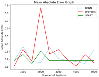
Figure 1. Mean absolute error graph
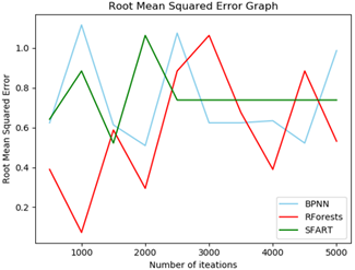
The groundwater quality grade prediction values obtained for the 3 models are presented in the following figures in terms of MAE and RMSE to observe the prediction error rate. As presented in Figure 1, the Mean Absolute Error values and Root Mean Squared Error values are provided. The horizontal axis represents the number of iterations and the vertical axis represents the MAE and RMSE values for the 3 models. From the Figure 1, it is observed that the MAE value is relatively low for the SFART model when compared with the other 2 models. The smaller MAE value indicates that the groundwater quality grade prediction values are closer to the true values. The RMSE values in the Figure 2 indicates that the SFART model produces better RMSE values than the other 2 models. From this study it is observed that the error rate is low indicating high performance of the SFART model in predicting the groundwater quality grade.
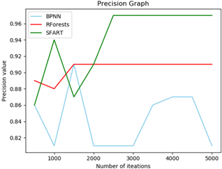
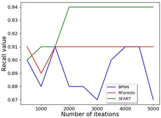
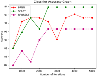
As presented in Figures 3-5, the groundwater quality prediction results are provided in terms of precision, recall, f score and classifier accuracy. These metrics are used to observe the groundwater quality grade prediction accuracy from the BPNN, R Forests and SFART models. The horizontal axis in the graphs represents the number of iterations and the vertical axis the graphs represent the accuracy scores for the precision, recall and f score values. From the Figure 6, it is observed that the SFART model outperforms the other 2 models in terms of better accuracy values. Hence, it is concluded that SFART model shows better performance than the other 2 models for groundwater quality grade classification and prediction. We observed that classifier accuracy is the best metric to classify the groundwater samples more accurately.
Figure 2. Root mean squared error graph
Figure 3. Precision graph
Figure 4. Recall graph
Figure 5. f score graph
Figure 6. Accuracy graph
In this paper, the potential of 3 ANN models Back propagation, Random Forests and Simplified Fuzzy ARTMAP are studied to predict the class label of groundwater samples. These models are implemented in the Python 3.7.4 programming language. From the experimental results, it is evident that the Simplified Fuzzy ARTMAP classifier has outperformed the BPNN and R Forest models in terms of number of iterations. The SFART classifier accuracy seems to be stable after 2500 iterations unlike BPNN and R Forests models. This work greatly helps the water quality monitoring stations to assess and classify the groundwater samples. In future, we intent to improve the SFART classifier by considering the relative weights of the groundwater quality parameters for more accurate groundwater grade assessment and classification process.
We thank Water Quality Monitoring Lab, RWS&S Sub-Division, Narsapuram, West Godavari, Andhra Pradesh, India, for giving the groundwater samples data and their permission to use the data in the present research work. We also thank Editor-in-Chief and the anonymous reviewers for their valuable suggestions to make this research article as an informative one.
|
ICMR |
Indian Council of Medical Research |
|
WQI |
Water Quality Index |
|
ANN |
artificial neural network |
|
BPNN |
Back propagation neural network |
|
SFART |
simplified fuzzy Adaptive Resonance Theory |
|
R forest |
random forest |
|
PCA |
principal component analysis |
|
pH |
potential of Hydrogen |
|
DO |
dissolved oxygen |
|
BOD |
biological oxygen demand |
|
TH |
total hardness |
|
TDS |
total dissolved solids |
|
T-Alk |
total alkalinity |
|
Pb |
Lead |
|
Cd |
Cadmium |
|
Cr |
Chromium |
|
Mn |
Manganese |
|
Fe |
Iron |
|
Zn |
Zinc |
|
Ni |
Nickel |
|
T-Alk |
Total alkalinity |
|
MAE |
mean absolute error |
|
RMSE |
root mean square error |
|
$\rho$ |
vigilance parameter |
|
$\varepsilon$ |
a samll number between 0 and 1. |
|
Subscripts |
|
|
Xi |
ith value of the sample |
|
Xmax |
maximum value of the x |
|
Xmin |
minimum value of the x. |
|
Tj |
activation function of the jth node |
|
Wj |
weights of the jth node |
[1] Horton, R.K. (1965). An index number system for rating water quality. Journal of Water Pollution Control Federation, 37(3): 300-306.
[2] Brown, R.M., Mc Clelland, N.I., Deininger, R.A., Tozer, R.G. (1970). Awater quality index-do we dare? Water Sew Works, 117: 339-343.
[3] Cude, C.G. (2001). Oregon water quality index: a tool for evaluating water quality management effectiveness. Journal of the American Water Resources Association, 37(1): 125-137. https://doi.org/10.1111/j.1752-1688.2001.tb05480.x
[4] Khwaja Anwar, M., Vanita, Aggarwal. (2014). Analysis of groundwater quality of Aligarh City, (India): Using water quality index. Current World Environment an International Research Journal of Environmental Science, 9(3): 851-857. http://dx.doi.org/10.12944/CWE.9.3.36
[5] Bureau of Indian Standards (BIS). 2012. Indian standard drinking water Specification. 2nd revision. IS: 10500. New Delhi, India: Bureau of Indian Standards.https://cpcb.nic.in/wqm/BIS_Drinking_Water_Specification.pdf.
[6] Gupta, A.K., Gupta, S.K., Patil, R.S. (2003). A comparison of water quality indices for coastal water. Journal of Environmental Science and Health, Part A, 38(11): 2711-2725. https://doi.org/10.1081/ESE-120024458
[7] Zotou, I., Tsihrintzis, V.A., Gikas, G.D. (2019). Performance of seven water quality indices (WQIs) in a Mediterranean river. Environmental Monitoring and Assessment, 191(8): 1-14. https://doi.org/10.1007/s10661-019-7652-4
[8] Uddin, M.G., Moniruzzaman, M., Khan, M. (2017). Evaluation of groundwater quality using CCME water quality index in the Rooppur Nuclear Power Plant Area, Ishwardi, Pabna, Bangladesh. American Journal of Environmental Protection, 5(2): 33-43. https://doi.org/10.12691/env-5-2-2
[9] Saleem, M., Hussain, A., Mahmood, G. (2016). Analysis of groundwater quality using water quality index: A case study of greater Noida (Region), Uttar Pradesh (UP), India. Cogent Engineering, 3(1): 1237927. https://doi.org/10.1080/23311916.2016.1237927
[10] Rajendran, R., Alice Emerenshiya, C., Dheenadayalan, M.S. (2018). Investigations on groundwater quality in Tiruchirappalli city, Tamilnadu, India. Journal of Sustainable Water Resources Management, 5: 599-609. https://doi.org/10.1007/s40899-018-0223-y
[11] Asadi, E., Isazadeh, M., Samadianfard, S., Ramli, M.F., Mosavi, A., Nabipour, N., Chau, K.W. (2019). Groundwater quality assessment for sustainable drinking and irrigation. Sustainability, 12(1). https://doi.org/10.3390/su12010177
[12] Verma, P., Singh, P.K., Sinha, R.R., Tiwari, A.K. (2020). Assessment of groundwater quality status by using water quality index (WQI) and geographic information system (GIS) approaches: A case study of the Bokaro district, India. Applied Water Science, 10(1): 1-16. https://doi.org/10.1007/s13201-019-1088-4
[13] Shankar, B.S., Raman, S. (2020). A novel approach for the formulation of modified water quality index and its application for groundwater quality appraisal and grading. Human and Ecological Risk Assessment: An International Journal, 26(10): 2812-2823. https://doi.org/10.1080/10807039.2019.1688638
[14] Krishna, A.K., Satyanarayanan, M., Govil, P.K. (2009). Assessment of heavy metal pollution in water using multivariate statistical techniques in an industrial area: a case study from Patancheru, Medak District, Andhra Pradesh, India. Journal of Hazardous Materials, 167(1-3): 366-373. https://doi.org/10.1016/j.jhazmat.2008.12.131
[15] Gulgundi, M.S., Shetty, A. (2016). Identification and apportionment of pollution sources to groundwater quality. Environmental Processes, 3(2): 451-461. https://doi.org/10.1007/s40710-016-0160-4
[16] Khuan, L.Y., Hamzah, N., Jailani, R. (2002). Prediction of water quality index (WQI) based on artificial neural network (ANN). Student Conference on Research and Development, Shah Alam, Malaysia, pp. 157-161. https://doi.org/10.1109/SCORED.2002.1033081
[17] Hao, Z.L., Zhang, Y.Y., Feng, M.Q. (2011). Water quality assessment based on BP network and its application. 2011 International Symposium on Water Resource and Environmental Protection, 2: 872-876. IEEE. https://doi.org/10.1109/iswrep.2011.5893150
[18] Wagh, V.M., Panaskar, D.B., Muley, A.A., Mukate, S.V., Lolage, Y.P., Aamalawar, M.L. (2016). Prediction of groundwater suitability for irrigation using artificial neural network model: A case study of Nanded tehsil, Maharashtra, India. Modeling Earth Systems and Environment, 2(4): 1-10. https://doi.org/10.1007/s40808-016-0250-3
[19] Kheradpisheha, Z., Talebib, A., Rafatia, L., Ghaneiana, M.T., Ehrampousha, M.H., (2015). Groundwater quality assessment using artificial neural network: A case study of Bahabad plain, Yazd, Iran. International Journal of Desert Research Centre. Winter and Spring, 20(1): 65-71. https://doi.org/10.22059/JDESERT.2015.54084
[20] Purkait, B., Kadam, S.S., Das, S.K. (2008). Application of artificial neural network model to study arsenic contamination in groundwater of Malda District, Eastern India. Journal of Environmental Informatics, 12(2): 140-149. https://doi.org/10.3808/jei.200800132
[21] Ganga Devi, S.V.S. (2019). Random forest advice for water quality prediction in the regions of Kadapa District. International Journal of Innovative Technology and Exploring Engineering, 8(6S4): 1464-1466. https://doi.org/10.35940/ijitee.F1298.0486S419
[22] Wang, X., Liu, T., Zheng, X., Peng, H., Xin, J., Zhang, B. (2018). Short-term prediction of groundwater level using improved random forest regression with a combination of random features. Applied Water Science, 8(5): 1-12. https://doi.org/10.1007/s13201-018-0742-6
[23] Hosseini-Moghari, S.M., Ebrahimi, K., Azarnivand, A. (2015). Groundwater quality assessment with respect to fuzzy water quality index (FWQI): An application of expert systems in environmental monitoring. Environmental Earth Sciences, 74(10): 7229-7238. https://doi.org/10.1007/s12665-015-4703-1
[24] Saberi Nasr, A., Rezaei, M., Dashti Barmaki, M. (2013). Groundwater contamination analysis using fuzzy water quality index (FWQI): Yazd province, Iran. Geopersia, 3(1): 47-55. https://doi.org/10.22059/JGEOPE.2013.31931
[25] Sahu, M., Mahapatra, S.S., Sahu, H.B., Patel, R.K. (2011). Prediction of water quality index using neuro fuzzy inference system. Water Quality, Exposure and Health, 3(3): 175-191. https://doi.org/10.1007/s12403-011-0054-7
[26] Dahіya, S., Sіngh, B., Gaur, S. (2007). Analysіs of groundwater quality using fuzzy synthetic evaluation. Journal of Hazardous Materials, 147(3): 938-946. https://doi.org/10.1016/j.jhazmat.2007.01.119
[27] Gharibi, H., Mahvi, A.H., Nabizadeh, R., Arabalibeik, H., Yunesian, M., Sowlat, M.H. (2012). A novel approach in water quality assessment based on fuzzy logic. Journal of Environmental Management, 112: 87-95. https://doi.org/10.1016/j.jenvman.2012.07.007
[28] Kiran Relangi, N.D.S.S., Chaparala, A., Sajja, R. (2019). Perspectives in water quality assessment. International Journal of Recent Technology and Engineering, 8(2S4): 7-11. https://doi:10.35940/ijrte.B1002.0782S419
[29] Agarwal, M., Singh, M., Hussain, J. (2020). Evaluation of groundwater quality for drinking purpose using different water quality indices in parts of Gautam Budh Nagar District, India. Asian Journal of Chemistry, 32(5): 1128-1138. https://doi.org/10.14233/ajchem.2020.22531
[30] Saen, F.R. (2009). The use of artificial neural networks for technology selection in the presence of both continuous and categorical data. World Applied Sciences Journal, 6: 1177-1189. https://doi.org/10.1016/j.amc.2005.09.037
[31] Tyagi, S., Sharma, B., Singh, P., Dobhal, R. (2013). Water quality assessment in terms of Water Quality Index. American Journal of Water Resources, 1(3): 11-15. https://https://doi.org/10.12691/ajwr‐1‐3‐3
[32] Rumelhart, D.E., Hinton, G.E., Williams, R.J. (1986). Learning representations by back-propagating errors. Nature, 323(6088): 533-536. https://doi.org/10.1038/323533a0
[33] Breiman, L. (2001). Random forests. Machine Learning, 45: 5-32. https://doi.org/10.1023/A:1010933404324
[34] Zadeh, L.A. (1965). Fuzzy sets. Inform Control, 8: 338-353. https://doi.org/10.1016/S0019-9958(65)90241-X
[35] Markuzon, R., Carpenter, G., Grossberg, S. (1992). Fuzzy ARTMAP: A neural network architecture for incremental supervised learning of analog multidimensional maps. IEEE Transactions on Neural Networks, 3(5): 698-713. https://doi.org/10.1109/72.159059
[36] Kasuba, T. (1993). Simplified fuzzy ARTMAP. AI Expert, 8(11): 18-25.