Andres A. Sánchez-Escalona* | Yanán Camaraza-Medina | Yoalbys Retirado-Mediaceja | Ever Góngora-Leyva
© 2021 IIETA. This article is published by IIETA and is licensed under the CC BY 4.0 license (http://creativecommons.org/licenses/by/4.0/).
OPEN ACCESS
Reliability of heat exchangers thermal analysis strongly depends on the equations selected to determine local convective heat transfer coefficients. Chosen analogy among momentum, heat and mass transfer also plays a remarkable role. Within this context, the aim of the study was to validate a novel approach to obtain mean forced convective film coefficients under single-phase non-laminar fluid flow conditions, inside tubes. It relied on a comprehensive Nusselt-number equation that is able to evolve into different functional forms according to Reynolds-Colburn, Prandtl and von Karman analogies. Parameters estimation was carried out through Genetic Algorithms. Applied experimental database was numerically obtained by Taler by solving the energy conservation equation for fully developed turbulent flow in tubes with constant wall heat flux. Application of the method provided a new correlation, valid for $0.1 \leq \operatorname{Pr} \leq 10^{3}$ and $3 \times 10^{3} \leq R e \leq 10^{6}$. Besides attaining a better fit to the experimental data as compared to benchmark expressions, it correlated very well with the results of reference models (Skupinski, Seban & Shimazaki, Gnielinski, Camaraza-Medina, Petukhov, and Sandall). The first assessment provided mean and maximum relative errors of 2.41% and 19.45%, respectively, while the second comparison resulted in deviations over the Nusselt number up to 20% in 92.59% of the data points. The implemented solution overcomes the drawbacks of non-linear and symbolic regression methods by allowing evolution of the regression function within a controlled mathematical environment. Future model improvements should investigate different fitting-intervals along with higher turbulence regions.
analogy, artificial intelligence, convection, correlation, genetic algorithms, heat exchanger, heat transfer
Engineers and researchers need proper heat transfer correlations to optimize the design and operation of heat exchangers. These equations are utilized for thermal analysis of the equipment, by applying the Logarithm Mean Temperature Difference (LMTD), Effectiveness–Number of Transfer Units (ε-NTU), Temperature Effectiveness (P-NTU), or any other method. They are a necessity for many project calculations or evaluation of industrial facilities [1-3]. Since the use of wrong or inexact correlations may result in under- or over-sizing of heat exchangers, poor selection of the operational ranges, as well as incorrect estimation of the fouling factors, the use of accurate Nusselt number equations is indispensable to ensure efficiency and profitability of the chemical process industries [4, 5].
Appropriate selection of the analogy among momentum, heat and mass transfer should not be ignored during experimental determination of internal convective heat transfer coefficients in tubular heat exchangers. It not only allows definition of the equation functional form, but also plays a significant role in accurateness of the results. This theory is based on description of the fluid flow through the continuity equations, the Navier-Stokes equations and boundary conditions, hence decoupling the mass species and energy expressions under constant property assumption. The experimental evidences and correspondence amongst both dimensionless expressions indicate that they are similar, which implies that solution of one of the processes conveys to resolution of the analogous phenomenon [6, 7].
Reynolds was the first researcher that realized the link between the energy transport processes. In 1874 he related the heat and momentum transfer for turbulent flows in straight round pipes. Chilton and Colburn improved his postulates in 1934, by extending its applicability to fluids with Prandtl and Schmidt numbers different from the unity $P r \neq 1$ and $S c \neq 1$ [8, 9].
This empirical adjustment to the original approach is often referenced as the Reynolds-Colburn analogy, which resulted in correlations with the mathematical structure of Eq. (1):
$Nu={{k}_{1}}\cdot R{{e}^{{{k}_{2}}}}\cdot P{{r}^{{{k}_{3}}}}$ (1)
where, Nu – Nusselt number; Re – Reynolds number; Pr – Prandtl number; ki– correlation adjustment coefficients.
Despite monomial power-type equations offers calculation simplicity, they introduce errors in the order of ±25%. In general terms; these correlations are not able to provide truthful approximations over a wide range of experimental data [5, 6, 10].
Prandtl modified the initial model in 1928, by assuming that the boundary layer is comprised by two zones: viscous and turbulent sublayers. He theorized that molecular transport rates prevail on the first region, while a turbulent transport rate does on the second. Correlations derived from this analogy take the Eq. (2) functional form [11]:
$Nu=\frac{\left( f/8 \right)\cdot \left( Re-{{k}_{4}} \right)\cdot Pr}{1+{{k}_{5}}\cdot \sqrt{f/8}\cdot \left( P{{r}^{{{k}_{6}}}}-1 \right)}$ (2)
In Eq. (2) f is the Darcy-Weisbach friction factor. Although Prandtl’s solution offers a significant improvement as compared to Reynolds analogy, because considering the viscous effects, his original equation diverges from experimental data for Pr ≠ 1 or Sc ≠ 1 [6, 7].
A few years later, in 1939, von Karman expanded Prandtl’s analogy by dividing the boundary layer into three zones: viscous, buffer, and turbulent core. He made assumptions alike his predecessor about the relative magnitude between molecular and turbulent transport rates on the viscous and turbulent sublayers, but incorporated the effects over the buffer region by supposing that viscous and turbulent rates were here of the same order of magnitude. The Nusselt number correlation deduced from this analogy is generically represented by Eq. (3) [12]:
$Nu=\frac{{{k}_{1}}\cdot R{{e}^{{{k}_{2}}}}\cdot Pr}{1+{{k}_{5}}\cdot R{{e}^{-0,1}}\cdot \left[ \left( Pr-1 \right)+\ln \left( \frac{5\text{ }Pr+1}{6} \right) \right]}$ (3)
The usage of a three-region model made the turbulent heat and mass transfer theory closer to the realistic flow conditions [13]. However, von Karman’s analogy becomes progressively inaccurate as Pr and Sc increase beyond 30 [6-8].
In spite of their limitations, Reynolds, Colburn, Prandtl and von Karman studies are mandatory references within the context under analysis. In this respect, such analogies are considered the major outcomes of the theory that correlates the heat exchange with friction factor for turbulent convective heat transfer modeling [14].
In most of the methods for characterization of the forced convective heat transfer inside tubes, the correlation functional form needs to be assumed a priori without an exhaustive analysis of the analogy that best describes the experimental data. Even though the mathematical function that relates the Nusselt number with the independent variables is generally selected on the basis of simplicity, compactness and common usage, it cannot be just justified according to these principles. This issue demands special attention, as it can significantly limit the reliability of calculated film coefficients [15, 16].
Despite several parameter estimation methods are applied to obtain heat transfer correlations from experimental data, as briefly summarized by Tam et al. [17, 18], there are only two approaches (according to the authors best knowledge) that eludes anticipated selection of the Nusselt-equation functional form. The first one is symbolic regression, performed through Genetic Programming algorithms, which not only allows determination of the equation constants, but also its mathematical structure [19-21].
However, the resultant expressions are aleatory, have a limited use in practical applications, and are deprived of a theoretical support. The second approach is referred here in as the ‘Nusselt-equation simulated evolution method’, and was devised to link relevant analogies among momentum, heat and mass transfer [18]. It automatically converges into the lowest-errors correlation, through successive modifications of the Nusselt number fitting function. Although physical meaning and generalization of obtained expressions were significantly improved as compared to symbolic regression, this scheme has only been tested versus synthetic data.
Considering previous research gaps, the objective of the actual study was to validate the ‘Nusselt-equation simulated evolution method’ through experimental data, by proposing new forced convective heat transfer correlations and comparing the results with other models that are applicable to single-phase non-laminar fluid flows inside tubes. Key expected contributions are:
The remaining part of this paper is organized as follows: Section 2 explains applied methodology and novelty of the proposed parameters estimation method; Section 3 shows most relevant results, in accordance with the study logical sequence; and Section 4 exposes main concluding remarks.
2.1 Applied methodology
2.1.1 Overview
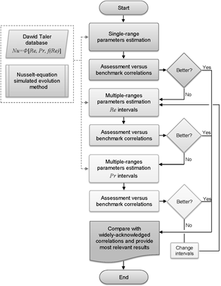
A progressive-approximation concept was applied on this research to determine the forced convective heat transfer correlation that best fits to the experimental data. It started with a single-range parameter estimation to determine the constants of the Nusselt-equation, and continued with estimation by batches for different intervals of the independent variables (i.e., the Reynolds and Prandtl numbers).
During each step, accurateness of the obtained Nusselt-equation to reproduce the experimental data was assessed versus benchmark correlations, and then moving forward until a highest precision is achieved. Once the appropriate convective heat transfer expression was selected, it was compared to widely-acknowledged correlations to validate this study results (see Figure 1). The parameter estimation method and the experimental database applied on this research are described on sections 2.2 and 2.3.
Correction factors for finite tube length and temperature-dependent fluid properties were neglected in all cases when comparing the correlations with experimental data.
2.1.2 Benchmark correlations
Only a few heat transfer models for pipe internal flows are valid in the transition and turbulent regions [22]. Within this context, three correlations were used to weight obtained expressions on every approximation step. The first one was Gnielinski’s [23], according to Eq. (4), which is one of the most recognized models worldwide.
Figure 1. Nusselt-equation parameter estimation methodology
Apart from its accuracy, the extensive application range $3 \times 10^{3}<R e<5 \times 10^{6}$, $0.5<\operatorname{Pr}<2 \times 10^{3}$, $0.025<\mu / \mu_{w}<12.5$, is an important feature of this equation, which couples heat transfer coefficient and friction factor compared with many other experimental correlations [14].
$Nu=\frac{\left( f/8 \right)\cdot (Re-1000)\cdot Pr}{1+12.7\sqrt{f/8}\quad\cdot \left( P{{r}^{2/3}}-1 \right)}\cdot {{K}_{L}}\cdot {{K}_{\mu }}$ (4)
where, μ – dynamic viscosity at fluid bulk temperature, Pa·s; μw – dynamic viscosity evaluated at wall temperature, Pa·s; KL and Kµ– finite tube length and viscosity correction factors, respectively. The model of Filonenko was suggested for calculation of the friction factor [24]:
$f={{(1.82\cdot \log Re-1.64)}^{-2}}$ (5)
The other two correlations were proposed by Taler [25], and selected as benchmarks since devised from the same database that this research used, thus having identical validity ranges $3 \times 10^{3} \leq R e \leq 10^{6}, 0.1 \leq \operatorname{Pr} \leq 10^{3}$. Eq. (6) functional form is based on Prandtl analogy, while Eq. (7) is a monomial power-type expression derived from the Reynolds-Colburn analogy:
$Nu=\frac{\left( f/8 \right)\cdot Re\cdot P{{r}^{1.0085}}}{1.076+12.4751\sqrt{f/8}\quad\cdot \left( P{{r}^{2/3}}-1 \right)}$ (6)
$Nu={{x}_{1}}\cdot R{{e}^{{{x}_{2}}}}\cdot P{{r}^{{{x}_{3}}}}$ (7)
where,
$[{{x}_{1}},{{x}_{2}},{{x}_{3}}]=\left\{ \begin{align} & [0.02155,\text{ }0.8018,\text{ }0.7095],\text{ if }0.1\le Pr\le 1 \\ & [0.01253,\text{ }0.8413,\text{ }0.6179],\text{ if }1<Pr\le 3 \\ & [0.00881,\text{ }0.8991,\text{ }0.3911],\text{ if 3}<Pr\le 1000 \\\end{align} \right.$
2.1.3 Correlations for further comparison
Six widely-acknowledged correlations were lastly used to appraise the proposed convective heat transfer equation. Its selection, besides aimed to cover the entire validity range of the applied experimental data, relied on the number of citations, recognition from the international scientific community, as well as accuracy level. These models are listed below:
The correlation of Skupinski is valid for $10^{2}<P e, 30<L / d$, and constant heat flux. This model is defined by Eq. (8) [26]:
$Nu=4.82+0.0185\cdot {{(Re\cdot Pr)}^{0.827}}$ (8)
where, L – tube length, m; d – tube inside diameter, m.
The correlation of Seban & Shimazaki is valid for $10^{2}<P e, 30<L / d$, and constant surface temperature. This model is defined by Eq. (9) [27]:
$Nu=5+0.025\cdot {{(Re\cdot Pr)}^{0.8}}$ (9)
The Equation of Petukhov represented by Eq. (10), pertinent for fully developed turbulent flows when $10^{4}<R e<5 \times 10^{6}$, $0.5<\operatorname{Pr}<2 \times 10^{3}$, $0.8<\mu / \mu_{w}<40$. This correlation is a reliable interpolation of approximate analytical solutions of momentum and energy equations for pipe flows at constant heat flux, if constant properties are assumed. Since predicting experimental results with an accuracy of 5-10%, this model is regularly used as a basis for comparisons that do not involve experimental data [28, 29].
$Nu=\frac{\left( f/8 \right)\cdot Re\cdot Pr}{1.07+12.7\sqrt{f/8}\quad\cdot \left( P{{r}^{2/3}}-1 \right)}$ (10)
Sandall et al. [30], given by Eq. (11), suitable for $10^{4}<R e<5 \times 10^{6}$, $0.5<\operatorname{Pr}<2 \times 10^{3}$, $0.025<\mu / \mu_{w}<12.5$. This correlation provides very good results for calculation of the average heat transfer coefficient in confined turbulent flows. Average errors of 8% are reported for medium viscosity fluids [6].
$Nu=\frac{\left( f/8 \right)\cdot Re\cdot Pr}{12.48\cdot P{{r}^{2/3}}-7.853\cdot P{{r}^{1/3}}+3.613\cdot \ln Pr+5.8+J}$ (11)
where,
$J=2.78\cdot \ln \left( \frac{1}{45}\cdot Re\cdot \sqrt{f/8} \right)$ (11a)
Gnielinski [23], according to Eq. (4), and applicable for $3 \times 10^{3}<R e<5 \times 10^{6}, 0.5<\operatorname{Pr}<2 \times 10^{3}$, $0.025<\mu / \mu_{w}<12.5$ as explained before. Camaraza-Medina et al. [31, 32], as per Eq. (12), projected for a much wider validity range: $2.4 \times 10^{3}<R e<8.2 \times 10^{6}, 0.65<\operatorname{Pr}<4.71 \times 10^{3}$, $0.006<\mu / \mu_{w}<177,2<L / d<420$.
$Nu=\frac{\left( Re-{{10}^{D}} \right)\cdot Pr}{A\cdot {{B}^{2}}-C\cdot B\cdot \left( 1-P{{r}^{2/3}} \right)}$ (12)
where,
$A=\left\{ \begin{align} & 75.44,\quad \quad if\ 2.4\times {{10}^{3}}<\operatorname{Re}<{{10}^{4}} \\ & 91.415,\quad \ \,if\ \operatorname{Re}\ge {{10}^{4}} \\\end{align} \right.$ (12a)
$B=\log \left( \frac{R{{e}^{0.56}}}{3.196} \right)$ (12b)
$C=\left\{ \begin{align} & 104,\quad \quad if\ 2.4\times {{10}^{3}}<\operatorname{Re}<{{10}^{4}} \\ & 116.74,\quad \ \,if\ \operatorname{Re}\ge {{10}^{4}} \\\end{align} \right.$ (12c)
$D=\left\{ \begin{align} & -0.027{{\left( \log \operatorname{Re} \right)}^{2}}+0.2\log \operatorname{Re}+2.63, \\ & \quad \quad \quad \quad \quad if\ 2.4\times {{10}^{3}}<\operatorname{Re}<{{10}^{4}} \\ & 0\ \,\quad \quad \ \quad \ \,if\ \operatorname{Re}\ge {{10}^{4}} \\\end{align} \right.$ (12d)
Note that, for simplicity, correction factors were omitted on previous expressions.
2.2 Nusselt-equation simulated evolution method
This method was recently devised by Sánchez-Escalona et al. [18], as a novel approach to obtain the mean heat transfer coefficients for single-phase non-laminar fluid flow inside tubes. It essentially consists on a comprehensive Nusselt-number equation, according to Eq. (13), that is able to evolve into three different functional forms derived from the analogies among momentum, heat and mass transfer as proposed by Reynolds-Colburn, Prandtl and von Karman. Evolution of Eq. (13) is simulated through Genetic Algorithms (GA), by a global iterative search of the individual (i.e., mathematical solution) that minimize deviations among expected (Nu) and calculated (Nu') Nusselt numbers.
In this manner not only the equation constants are determined, but also the correlation functional form with best fitting to the experimental data. This approach is considered by the authors as a hybrid method between parametric and symbolic regression, since adaptation of the regression function is allowed, occurring within a controlled environment to avoid randomness of the solution, poor generalization and lack of physical sense.
Previous expression involves eight parameters (b1, b2, d1, d2, c1, c2, c3 and c4) that define the coefficients and functional form of the Nusselt number correlation. The first two only admit binary values, according to Eq. (13a) and Eq. (13b), and were conceived to identify the momentum, heat and mass transfer analogy that best describes the experimental data:
$Nu'=\frac{{{c}_{1}}\cdot {{\left( \frac{f}{8} \right)}^{{{b}_{1}}\cdot {{b}_{2}}}}\cdot \left( R{{e}^{{{c}_{2}}^{^{(1-{{b}_{1}}\cdot {{b}_{2}})}}}}-{{b}_{1}}\cdot {{b}_{2}}\cdot {{c}_{3}} \right)\cdot P{{r}^{{{d}_{1}}^{(1-{{b}_{1}})}}}}{{{\left\{ 1+{{c}_{4}}\cdot R{{e}^{-0.1(1-{{b}_{2}})}}\quad\cdot {{\left( \frac{f}{8} \right)}^{0.5\text{ }{{b}_{2}}}}\left[ \left( P{{r}^{{{d}_{2}}}}-1 \right)+\left( 1-{{b}_{2}} \right)\cdot \ln \left( \frac{5\text{ }Pr+1}{6} \right) \right] \right\}}^{{{b}_{1}}}}}$ (13)
$b_{1}=\left\{\begin{array}{l}0, \text { if Reynolds analogy, } \\ 1, \text { if superior analogy (Prandtl or von Karman). }\end{array}\right.$ (13a)
$b_{2}=\left\{\begin{array}{l}0, \text { if von Karman analogy, } \\ 1, \text { if Prandtl analogy. }\end{array}\right.$ (13b)
The second set, as defined by Eq. (13c) and Eq. (13d), acquires discrete values associated with the Prandtl number exponent:
${{d}_{1}}=\left\{ 1/3;\text{ }2/5 \right\}$ (13c)
${{d}_{2}}=\left\{ 2/3;\text{ 1} \right\}$ (13d)
Remaining parameters are curve-fitting correlation coefficients, which were intended to admit real values within the intervals described by Eq. (13e) to Eq. (13h):
$0<c_{1} \leq 1$ (13e)
$0<c_{2} \leq 1$ (13f)
$0 \leq c_{3} \leq 1500$ (13g)
$0<c_{4} \leq 20$ (13h)
Unknown coefficients appearing in the approximating function were determined by means of GA, using a MATLAB® R2013a environment. Options and parameters related to the algorithm configuration are summarized in Table 1.
Table 1. GA configuration
|
Category |
Parameter |
Value |
|
Population |
Population size |
1500 |
|
Fitness scaling |
Scaling function |
Rank |
|
Selection |
Selection function |
Stochastic uniform |
|
Reproduction |
Elite count |
1 |
|
|
Crossover fraction |
0.5 |
|
Mutation |
Mutation function |
Constraint dependent |
|
Crossover |
Crossover function |
Scattered |
|
Migration |
Fraction |
0.2 |
|
|
Interval |
20 |
|
Constraints |
Initial penalty |
10 |
|
|
Penalty factor |
100 |
|
Stop criteria |
Generations |
300 |
|
|
Time limit |
∞ |
|
|
Fitness limit |
-∞ |
|
|
Stall generations |
50 |
|
|
Stall time limit |
∞ |
|
|
Function tolerance |
10-24 |
|
|
Nonlinear constraint tolerance |
10-24 |
Even though the maximum relative error was the fitness function recommended on the initial research [18], it was hereby determined that minimization of the sum of squared errors, as expressed in Eq. (14), provided superior consistency and faster results.
$\underset{\mathbf{X},\mathbf{Y}}{\mathop{\arg \min }}\,\left\{ \sum\limits_{i=1}^{n}{\left[ N{{u}_{i}}-Nu{{'}_{i}}(\mathbf{X},\mathbf{Y}) \right]}{{\text{ }}^{2}} \right\}$ (14)
where, Nu– experimental Nusselt number value; Nu' – calculated Nusselt number value, as function of vectors X and Y; n – number of data points. Vector X includes the parameters to be estimated by the GA, while Y is comprised by the values of the independent variables.
2.3 Nusselt number database
The experimental database used on this study was obtained by Taler [22, 25]. He predicted the Nusselt numbers as a function of the Reynolds and Prandtl numbers by solving the energy conservation equation for fully developed turbulent flow in tubes with constant wall heat flux:
$\rho \cdot {{c}_{P}}\cdot \bar{u}\cdot \frac{\partial \overline{T}}{\partial x}=\frac{1}{r}\frac{\partial }{\partial r}(r\cdot q)$ (15)
where, ρ – fluid density, kg/m3; cP – specific heat at constant pressure, J/(kg·K); $\bar{u}$ – time averaged velocity, m/s; $\overline{T}$ – time averaged temperature, K; x – cartesian coordinate, m;r – radial coordinate, m; q– heat flux density, W/m2. The heat flux comprises the molecular and turbulent components:
$q=(k+\rho \cdot {{c}_{P}}\cdot {{\varepsilon }_{q}})\frac{\partial \overline{T}}{\partial r}$ (16)
where, k – thermal conductivity, W/(m·K); εq – eddy diffusivity for heat transfer, m2/s. The authors applied the finite difference method to solve Eq. (15) subject to the following boundary conditions:
${{\left. k\cdot \frac{\partial \overline{T}}{\partial r} \right|}_{r={{r}_{w}}}}={{q}_{w}}$ (17a)
${{\left. \left[ \frac{\partial \overline{T}}{\partial r} \right]\text{ } \right|}_{r=0}}=0$ (17b)
${{\left. \overline{T}\text{ } \right|}_{x=0}}={{\left. {{T}_{m}}^{{}} \right|}_{x=0}}$ (17c)
where, rw – tube inner radius, m; qw – wall heat flux, W/m2; Tm – mass averaged bulk temperature, K, computed through Eq. (18).
${{T}_{m}}(x)=\frac{2}{{{r}_{w}}^{2}\cdot {{u}_{m}}}\int\limits_{0}^{{{r}_{w}}}{\bar{u}(r)}\cdot \bar{T}(x,r)\cdot r\text{ }dr$ (18)
where, um – mean velocity, m/s.
The time averaged velocity profile $\bar{u}(r)$ in the tube cross-section was necessary to determine the fluid temperature distribution. Hence, Reichardt’s empirical relationship was applied to calculate the eddy diffusivity for momentum transfer ετ and the time averaged fluid velocity $\bar{u}$[33]. According to Taler [10], this solution is straightforward and accurate.
Next, the Nusselt number was determined based on the temperature distribution using Eq. (19):
$Nu=\frac{2\cdot {{q}_{w}}\cdot {{r}_{w}}}{k\left( {{\left. T \right|}_{r={{r}_{w}}}}-{{T}_{m}} \right)}$ (19)
The Nusselt number was evaluated for various Reynolds and Prandtl numbers, ranging from $3 \times 10^{3}$ to $10^{6}$ and 0.1 to $10^{3}$ respectively (the results are reproduced on Table 2).
Table 2. Nusselt number as a function of the Reynolds and Prandtl numbers [10, 22, 25]
|
Pr |
Re |
|||||||||
|
$3 \times 10^{3}$ |
$5 \times 10^{3}$ |
$7.5 \times 10^{3}$ |
$10^{4}$ |
$3 \times 10^{4}$ |
$5 \times 10^{4}$ |
$7.5 \times 10^{4}$ |
$10^{5}$ |
$3 \times 10^{5}$ |
$10^{6}$ |
|
|
0.1 |
7.86 |
9.42 |
11.13 |
12.69 |
22.76 |
31.02 |
40.20 |
48.62 |
104.68 |
256.61 |
|
0.2 |
9.41 |
11.86 |
14.58 |
17.08 |
33.53 |
47.23 |
62.59 |
76.78 |
172.57 |
437.11 |
|
0.5 |
12.65 |
16.96 |
21.81 |
26.31 |
56.55 |
82.31 |
111.63 |
138.97 |
327.20 |
860.91 |
|
0.71 |
14.32 |
19.60 |
25.57 |
31.12 |
68.78 |
101.16 |
138.18 |
172.84 |
413.35 |
1102.29 |
|
1 |
16.22 |
22.61 |
29.86 |
36.61 |
82.91 |
123.04 |
169.15 |
212.50 |
515.41 |
1391.88 |
|
3 |
24.43 |
35.57 |
48.39 |
60.47 |
145.31 |
220.65 |
308.45 |
391.85 |
987.68 |
2764.63 |
|
5 |
29.56 |
43.64 |
59.94 |
75.36 |
184.68 |
282.64 |
397.43 |
506.89 |
1295.71 |
3677.45 |
|
7.5 |
34.34 |
51.15 |
70.68 |
89.21 |
221.38 |
340.53 |
480.68 |
614.66 |
1586.18 |
4544.73 |
|
10 |
38.16 |
57.14 |
79.24 |
100.25 |
250.64 |
386.73 |
547.14 |
700.78 |
1818.99 |
5242.89 |
|
12.5 |
41.40 |
62.20 |
86.47 |
109.56 |
275.31 |
425.71 |
603.25 |
773.51 |
2015.88 |
5834.61 |
|
15 |
44.23 |
66.62 |
92.78 |
117.70 |
296.85 |
459.72 |
652.22 |
836.98 |
2187.81 |
6352.24 |
|
30 |
56.73 |
86.09 |
120.53 |
153.40 |
391.25 |
608.73 |
866.75 |
1115.04 |
2941.80 |
8624.88 |
|
50 |
67.98 |
103.56 |
145.36 |
185.32 |
475.39 |
741.46 |
1057.70 |
1362.53 |
3612.61 |
10647.89 |
|
100 |
86.64 |
132.44 |
186.35 |
237.96 |
613.70 |
959.44 |
1371.11 |
1768.51 |
4711.28 |
13959.35 |
|
200 |
110.11 |
168.69 |
237.71 |
303.83 |
786.27 |
1231.01 |
1761.37 |
2273.65 |
6076.39 |
18067.10 |
|
1000 |
190.70 |
292.75 |
413.17 |
528.61 |
1373.01 |
2153.24 |
3085.03 |
3986.35 |
10692.06 |
31968.41. |
3.1 Single-range parameters estimation
The full range of experimental data $0.1 \leq P r \leq 10^{3}$ and $3 \times 10^{3} \leq R e \leq 10^{6}$ was used at once, on a first attempt to propose a convective heat transfer correlation for single-phase transition and turbulent fluid flow conditions, inside tubes. Application of the ‘Nusselt-equation simulated evolution method’ provided the following results (see Table 3).
When substituting computed coefficients into Eq. (13), the resultant correlation took the following form:
$Nu'=\frac{0.89\cdot \left( f/8 \right)\cdot \left( Re-136.2 \right)\cdot Pr}{1+10.478\cdot \sqrt{f/8}\quad\cdot \left( P{{r}^{2/3}}-1 \right)}$ (20)
In spite of the strong linear association that was determined through Eq. (20), by comparing the Nusselt number calculated values (Nu') against the reference ones (Nu), the more accurate results were reported for Eq. (6) suggested by Taler. In contrast, power-type correlations like Taler’s Eq. (7) were confirmed less appropriate to reproduce experimental results over a broad range of the independent variables (see Table 4).
Table 3. Single-range parameter estimation results
|
Variables |
|
Algorithm runs |
||||
|
|
1 |
2 |
3 |
4 |
5 |
|
|
Computed coefficients |
b1 |
1 |
1 |
1 |
1 |
1 |
|
b2 |
1 |
1 |
1 |
1 |
1 |
|
|
d1 |
2/5 |
1/3 |
2/5 |
2/5 |
2/5 |
|
|
d2 |
2/3 |
2/3 |
2/3 |
2/3 |
2/3 |
|
|
c1 |
0.89 |
0.89 |
0.89 |
0.89 |
0.89 |
|
|
c2 |
0.8856 |
0.2049 |
0.3322 |
1.0000 |
0.1721 |
|
|
c3 |
136.2 |
136.2 |
136.2 |
136.2 |
136.2 |
|
|
c4 |
10.478 |
10.478 |
10.478 |
10.478 |
10.478 |
|
|
Algorithm performance |
fobj |
98618 |
98618 |
98618 |
98618 |
98618 |
|
i |
300 |
288 |
241 |
192 |
300 |
|
|
sc1 |
I |
II |
II |
II |
I |
|
Notes: 1 Stop criteria:
I. Maximum number of generations exceeded;
II. Average change in the fitness value less than options.
where, fobj – objective function value once the algorithm stops; i – number of iterations.
Table 4. Assessment of Eq. (20) vs. benchmark correlations
|
Correlation |
Error indexes |
|||
|
R2 |
eave |
e max |
SSE |
|
|
This study, Eq. (20) |
0.999949 |
6.696 |
56.612 |
9.86·104 |
|
Gnielinski, Eq. (4) |
0.999398 |
10.652 |
42.013 |
8.63 106 |
|
Taler, Eq. (6) |
0.999985 |
4.307 |
37.208 |
3.06·104 |
|
Taler, Eq. (7) |
0.998721 |
11.102 |
67.154 |
2.50·106 |
where, R2 – coefficient of determination; eave – mean relative error,%; e max – maximum relative error,%; SSE – sum of squared errors. Utilized statistical and error metrics are described in Appendix A.
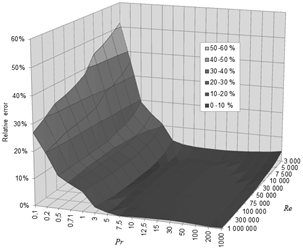
A 3D plot of the relative errors introduced by Eq. (20), as function of Prandtl and Reynolds numbers, shows larger deviations for $\operatorname{Pr} \leq 3$ and $R e<10^{4}$, with the first variable exerting the greatest influence (Figure 2).
3.2 Two Re-intervals parameters estimation
Regression by intervals is a common practice during experimental determination of convective heat transfer coefficients. In this respect, authors as Camaraza-Medina et al. [31, 32] performed parameters estimation for different ranges of the Reynolds number, comprehending that the flow regime have a direct impact on heat transfer intensification. Besides, some of the theories that correlate momentum, heat and mass transfer for turbulent flows are based on a velocity profile approach [34-36].
Figure 2. Relative errors 3D plot for Eq. (20)
Taking the above into consideration, a second approximation of the experimental data was carried out by batches, selecting two intervals of the Reynolds number: $3 \times 10^{3} \leq \operatorname{Re}<10^{4} \quad$ and $\quad 10^{4} \leq \operatorname{Re} \leq 10^{6}$. Parameters estimation results are shown below (see Tables 5 and 6).
Substitution of computed coefficients into Eq. (13) provided the following expression:
$Nu'=\frac{{{y}_{1}}\cdot \left( f/8 \right)\cdot \left( Re-{{y}_{2}} \right)\cdot Pr}{1+{{y}_{3}}\cdot \sqrt{f/8}\quad\cdot \left( P{{r}^{2/3}}-1 \right)}$ (21)
where,
$[{{y}_{1}},{{y}_{2}},{{y}_{3}}]=\left\{ \begin{align} & [0.9052,\text{ 7}\text{.80},\text{ 1}0.752],\text{ if }3\cdot {{10}^{3}}\le Re<{{10}^{4}} \\ & [0.8902,\text{ 243}\text{.75},\text{ 10}\text{.478}],\text{ if 1}{{\text{0}}^{\text{4}}}\le Re\le {{10}^{6}} \\\end{align} \right.$
Table 5. First Re-interval parameters estimation results
|
Variables |
|
Algorithm runs |
||||
|
|
1 |
2 |
3 |
4 |
5 |
|
|
Computed coefficients |
b1 |
1 |
1 |
1 |
1 |
1 |
|
b2 |
1 |
1 |
1 |
1 |
1 |
|
|
d1 |
2/5 |
2/5 |
1/3 |
1/3 |
2/5 |
|
|
d2 |
2/3 |
2/3 |
2/3 |
2/3 |
2/3 |
|
|
c1 |
0.9052 |
0.9052 |
0.9052 |
0.9052 |
0.9052 |
|
|
c2 |
0.7938 |
0.2427 |
0.5683 |
0.5406 |
0.4583 |
|
|
c3 |
7.8 |
7.8 |
7.8 |
7.65 |
7.8 |
|
|
c4 |
10.752 |
10.752 |
10.752 |
10.752 |
10.752 |
|
|
Algorithm performance |
fobj |
287.39 |
287.39 |
287.39 |
287.39 |
287.39 |
|
i |
246 |
218 |
204 |
176 |
275 |
|
|
sc1 |
II |
II |
II |
II |
II |
|
Even when Eq. (21) provided slightly better results as compared to Eq. (20), accuracy of Taler’s Eq. (6) remains the higher to this point (see Table 7).
Table 6. Second Re-interval parameters estimation results
|
Variables |
|
Algorithm runs |
||||
|
|
1 |
2 |
3 |
4 |
5 |
|
|
Computed coefficients |
b1 |
1 |
1 |
1 |
1 |
1 |
|
b2 |
1 |
1 |
1 |
1 |
1 |
|
|
d1 |
2/5 |
2/5 |
2/5 |
1/3 |
1/3 |
|
|
d2 |
2/3 |
2/3 |
2/3 |
2/3 |
2/3 |
|
|
c1 |
0.8902 |
0.8902 |
0.8902 |
0.8902 |
0.8902 |
|
|
c2 |
0.9969 |
0.4758 |
0.9996 |
1.0000 |
0.4361 |
|
|
c3 |
243.75 |
243.75 |
243.75 |
243.75 |
243.75 |
|
|
c4 |
10.478 |
10.478 |
10.478 |
10.478 |
10.478 |
|
|
Algorithm performance |
fobj |
97996 |
97996 |
97996 |
97996 |
97996 |
|
i |
300 |
300 |
300 |
216 |
194 |
|
|
sc1 |
I |
I |
I |
II |
II |
|
Table 7. Assessment of Eq. (21) vs. benchmark correlations
|
Correlation |
Error indexes |
|||
|
R2 |
eave |
e max |
SSE |
|
|
This study, Eq. (21) |
0.999949 |
6.286 |
46.293 |
9.82·104 |
|
Gnielinski, Eq. (4) |
0.999398 |
10.652 |
42.013 |
8.63·106 |
|
Taler, Eq. (6) |
0.999985 |
4.307 |
37.208 |
3.06·104 |
|
Taler, Eq. (7) |
0.998721 |
11.102 |
67.154 |
2.50·106 |
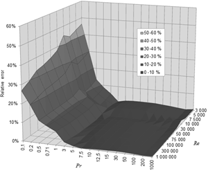
Figure 3. Relative errors 3D plot for Eq. (21)
3D plot of the relative errors introduced by Eq. (21) still exposes sudden deviations for low Prandtl numbers (see Figure 3). Potential reasons behind this outcome are the influence of this variable over the exponents of the Reynolds and Prandtl numbers, as well as the distinctive thermal behavior of liquid metals and analogous fluids (Pr<< 1).
As confirmed by Gnielinski [37] and Taler [10], power exponents at the Reynolds and Prandtl numbers strongly depend on the Prandtl number in turbulent flow. If Pr is smaller than one, power exponents with Re and Pr are close to each other. Besides, Taler highlighted that the Re exponent increases with the Prandtl number, while the Pr exponent responds inversely.
On the other hand, in low Prandtl-number fluids the contribution of the molecular thermal conduction to the total heat transfer is higher than other streams. Since having high thermal conductivity coefficients, thus very low molecular Pr that result in a much thicker thermal boundary layer as compared to the hydrodynamic one, it becomes difficult to correlate them concurrently with moderate and high Prandtl-number fluids [6, 38].
3.3 Two Pr-number intervals parameters estimation
Despite a few researchers tackled heat transfer problems by examining different ranges of the Reynolds number, others like Dalkilic & Wongwises [39], Gnielinski [23] and Taler [10] proposed film coefficient correlations based on Prandtl-number intervals. Likewise, it is noteworthy that accurate models like Polley’s [40], Sleicer-Rouse’s [41] and Sandall et al. [30] are supported on correlations where the Prandtl number have a significant influence as independent variable.
Therefore, and according to this study methodology, next approximation of the experimental data was carried out by batches over the Prandtl number: $0.1 \leq \operatorname{Pr} \leq 3$ and $3<\operatorname{Pr} \leq 10^{3}$. Parameters estimation results are summarized below (see Tables 8 and 9).
Table 8. First Pr-interval parameters estimation results
|
Variables |
|
Algorithm runs |
||||
|
|
1 |
2 |
3 |
4 |
5 |
|
|
Computed coefficients |
b1 |
1 |
1 |
1 |
1 |
1 |
|
b2 |
1 |
1 |
1 |
1 |
1 |
|
|
d1 |
1/3 |
2/5 |
2/5 |
1/3 |
1/3 |
|
|
d2 |
2/3 |
2/3 |
2/3 |
2/3 |
2/3 |
|
|
c1 |
0.9713 |
0.9713 |
0.9713 |
0.9713 |
0.9713 |
|
|
c2 |
0.5581 |
0.9997 |
0.7473 |
0.3704 |
0.9978 |
|
|
c3 |
205.05 |
205.05 |
205.05 |
205.05 |
205.05 |
|
|
c4 |
12.952 |
12.952 |
12.952 |
12.952 |
12.952 |
|
|
Algorithm performance |
fobj |
2177 |
2177 |
2177 |
2177 |
2177 |
|
i |
300 |
300 |
300 |
195 |
246 |
|
|
sc1 |
I |
I |
I |
II |
II |
|
Table 9. Second Pr-interval parameters estimation results
|
Variables |
|
Algorithm runs |
||||
|
|
1 |
2 |
3 |
4 |
5 |
|
|
Computed coefficients |
b1 |
1 |
1 |
1 |
1 |
1 |
|
b2 |
1 |
1 |
1 |
1 |
1 |
|
|
d1 |
2/5 |
1/3 |
2/5 |
2/5 |
2/5 |
|
|
d2 |
2/3 |
2/3 |
2/3 |
2/3 |
2/3 |
|
|
c1 |
0.8761 |
0.8761 |
0.8762 |
0.8761 |
0.8761 |
|
|
c2 |
0.8811 |
0.8422 |
0.7853 |
0.3137 |
0.3137 |
|
|
c3 |
147.3 |
147.3 |
147.3 |
147.3 |
147.3 |
|
|
c4 |
10.3 |
10.3 |
10.3 |
10.3 |
10.3 |
|
|
Algorithm performance |
fobj |
36670 |
36670 |
36670 |
36670 |
36670 |
|
i |
278 |
300 |
189 |
263 |
213 |
|
|
sc1 |
II |
I |
II |
II |
II |
|
Substitution of the above coefficients into Eq. (13) produced the following Nusselt number expression:
$Nu'=\frac{{{z}_{1}}\cdot \left( f/8 \right)\cdot \left( Re-{{z}_{2}} \right)\cdot Pr}{1+{{z}_{3}}\cdot \sqrt{f/8}\quad\cdot \left( P{{r}^{2/3}}-1 \right)}$ (22)
where,
$[{{z}_{1}},{{z}_{2}},{{z}_{3}}]=\left\{ \begin{align} & [0.9713,\text{ 205}\text{.05},\text{ 12}\text{.9}52],\text{ if }0.1\le Pr\le 3 \\ & [0.8761,\text{ 147}\text{.30},\text{ 10}\text{.300}],\text{ if 3}<Pr\le 1000 \\\end{align} \right.$
The resultant convective heat transfer correlation, given by Eq. (22), provided a better fit to the reference data (Nu) as compared to benchmark expressions (Table 10). Unlike the other equations, relative errors were lower than 20% for all data points (Figure 4).
Figure 4. Relative errors 3D plot for Eq. (22)
Table 10. Assessment of Eq. (22) vs. benchmark correlations
|
Correlation |
Error indexes |
|||
|
R2 |
eave |
e max |
SSE |
|
|
This study, Eq. (22) |
0.999984 |
2.409 |
19.446 |
3.03·104 |
|
Gnielinski, Eq. (4) |
0.999398 |
10.652 |
42.013 |
8.63·106 |
|
Taler, Eq. (6) |
0.999985 |
4.307 |
37.208 |
3.06·104 |
|
Taler, Eq. (7) |
0.998721 |
11.102 |
67.154 |
2.50·106 |
The constant c4 in Eq. (13) is related to the dimensionless velocity at the hypothetical distance from the tube surface to the boundary limit between the viscous (laminar) sublayer and the turbulent core. It depends on the viscous sublayer thickness and was expected from c4 = 5 for the three-sublayers model of von Karman to c4 = 11.7 for the two-zone boundary layer theory of Prandtl [22]. Despite slightly outside of the theoretical range, the results from this study c4 = z3 ={12.952; 10.300} were close to the coefficient 12.475 found by Taler [25]. In both cases, the additive form of the denominator arose from the two resistances in series of the Prandtl model for momentum and energy transfer [35].
It was remarkable that all runs of the ‘Nusselt-equation simulated evolution method’converged into a correlation that corresponds to Prandtl analogy. This emphasize that monomial power-type correlations based on Reynolds analogy do not provide good approximations, since assumed that the turbulent transport rates were much greater than the molecular transport rates, neglecting the later. The viscous effects are significant and can make comparable or even greater contributions than the turbulent effects in the near-wall region. It also underlines that Nusselt-number functional forms according to von Karman analogy are neither accurate if the studied data points include high Prandlt numbers. Deviations beyond Pr= 10 were attributed to the assumption of a fixed boundary between this model sublayers, independent of Reynolds and Prandtl numbers [6-8, 36].
3.4 Comparison with other correlations
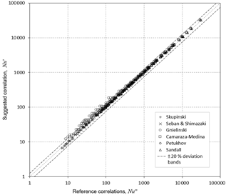
Considering previous results, Eq. (22) is recommended for calculation of the mean convective heat transfer coefficient for single-phase transition and turbulent fluid flow conditions, inside tubes. Besides accurately describing the experimental database used for this study, computed Nusselt number values agreed very well with those obtained through six known correlations, those of Skupinski et al, Seban & Shimazaki, Gnielinski, Camaraza-Medina et al., Nalavade et al. and Sandall et al (see Figure 5). The selected models are the widely-acknowledged correlations in the technical literature [26-32].
Figure 5. Scatter plot for computed Nu values
The relative deviations amongst Nusselt number values, calculated by Eq. (23), were used as a performance metric for quantitative comparison of the suggested correlation versus the reference ones:
${{d}_{Nu}}=\frac{\left| Nu''-Nu' \right|}{Nu''}\text{ }\cdot 100\text{ }%$ (23)
where, dNu – relative deviation over the dependent variable, %; Nu'– Nusselt number value calculated by means of Eq. (22); Nu'' – Nusselt number value calculated with the selected models.
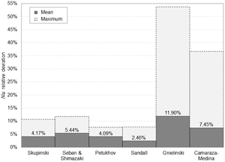
Owing that mean divergences were lower than 12% (see Figure 6), besides not exceeding 20% differences in 92.59% of the data points (see Table 11), this research correlation is considered appropriate for academic purposes and practical applications within the studied validity ranges: $3 \times 10^{3} \leq R e \leq 10^{6}$ and $0.1 \leq \operatorname{Pr} \leq 10^{3}$.
Figure 6. Relative deviations amongst Nu values
Table 11. Relative deviations percentage distribution
|
Relative deviation range |
Data points percent |
Cumulative percent |
|
0%<dNu ≤ 10% |
85.55 |
85.55 |
|
10%<dNu ≤ 20% |
7.04 |
92.59 |
|
20%<dNu ≤ 30% |
2.85 |
95.44 |
|
30%<dNu ≤ 40% |
2.66 |
98.10 |
|
40%<dNu ≤ 50% |
0.95 |
99.05 |
|
50%<dNu< 55% |
0.95 |
100.00 |
The largest deviations were found when comparing Eq. (22) versus the results from Gnielinski equation, since heat transfer modeling of the transitional flow zone is not as predictable as the turbulent regime. At one side, the lack of experimental data is most likely the reason for limited understanding and little design information about the transitional flow region, so it is yet considered a metastable and complicated zone [42]. At the other side, contemporary review of Gnielinski equation indicated a considerable amount of scatter (at least ±20%), presumably due to the antiquity of the data he used and the absence of modern instrumentation [43, 44].
Eq. (22) can be generalized to a tube of finite length and streams having large property variations due to remarkable temperature differences, by introducing two well-known correction factors [25, 37]:
$Nu'=\frac{{{z}_{1}}\cdot \left( f/8 \right)\cdot \left( Re-{{z}_{2}} \right)\cdot Pr}{1+{{z}_{3}}\cdot \sqrt{f/8}\quad\cdot \left( P{{r}^{2/3}}-1 \right)}\cdot \left[ 1+{{\left( \frac{d}{L} \right)}^{2/3}} \right]\cdot {{\left( \frac{Pr}{P{{r}_{w}}} \right)}^{0.11}}$ (24)
A correction based on temperature rather than the Prandtl number ratio (right-end multiplier) is recommended for gases [25, 37]:
${{K}_{\mu }}={{\left( \frac{{{T}_{b}}}{{{T}_{w}}} \right)}^{a}}$ (25)
where, Prw – Prandtl number evaluated at wall temperature, Tb – bulk temperature, K; Tw – wall temperature, K; a – correction factor exponent, equals to 0 for cooling and 0.45 for heating. While the last value was correlated by Gnielinski for 0.5 <(Tb/Tw)<1.0, there are other recommendations in the literature [45].
Despite the boundary condition assumed to gather the experimental database, recommended correlation can be used for either uniform wall heat flux or uniform wall temperature applications, if Re>104. While in the laminar and transitional flow regimes the boundary condition has a significant influence on the heat transfer characteristics, turbulent flow is practically insensitive to the different conditions [46-52].
An approximation-by-intervals methodology was applied to obtain forced convective heat transfer film coefficients, which allowed experimental validation of the ‘Nusselt-equation simulated evolution method’. As a result, a new correlation with the form Eq. (22b) was proposed for single-phase non-laminar fluid flows inside tubes. Its validity ranges are $3 \times 10^{3} \leq \operatorname{Re} \leq 10^{6}$ and $0.1 \leq \operatorname{Pr} \leq 10^{3}$.
This expression provided a better fit to the experimental data as compared to selected benchmarks (Taler’s and Gnielinski equations). Calculated coefficient of determination confirmed that 99.9984% of the Nusselt number variability was explained by the model. Relative errors averaged 2.409%, while attaining the maximum at 19.446%. These deviations fit well within engineering acceptable ranges.
Current study results were also compared with the outputs of selected models. The larger differences were found versus Gnielinski and Camaraza-Medina equations, over the range $3 \times 10^{3}<R e<10^{4}$, mainly attributable to uncertainties within the transition flow region. Nevertheless, given that deviations between calculated and reference Nusselt numbers did not exceed 20% in 92.59% of the data points, Eq. (22) is recommended for educational and practical applications.
Although regression by batches over Prandtl number ranges provided better results as compared to Reynolds number ranges, selection of the regression intervals shall be studied in more details. Further model improvements should also consider additional data points, in order to include higher turbulence regions $10^{6} \leq R e \leq 5 \times 10^{6}$ or beyond.
|
$a$ |
exponent in Eq. (25) |
|
${{b}_{1}}$, ${{b}_{2}}$, ${{c}_{1}}$, ${{c}_{2}}$, ${{c}_{3}}$, ${{c}_{4}}$, ${{d}_{1}}$,${{d}_{2}}$… |
regression parameters in Eq. (13) |
|
${{c}_{P}}$ |
specific heat at constant pressure, J/(kg·K) |
|
$d$ |
tube inside diameter, m |
|
${{d}_{Nu}}$ |
relative deviation over the dependent variable,% |
|
${{e}_{ave}}$ |
mean relative error,% |
|
${{e}_{max}}$ |
maximum relative error,% |
|
$f$ |
Darcy-Weisbach friction factor |
|
${{f}_{obj}}$ |
objective function value |
|
$i$ |
number of iterations |
|
$k$ |
fluid thermal conductivity, W/(m·K) |
|
${{k}_{i}}$ |
correlation adjustment coefficients |
|
${{K}_{L}}$ |
finite tube length correction factor |
|
${{K}_{\mu }}$ |
viscosity correction factor |
|
$L$ |
tube length, m |
|
$n$ |
number of data points |
|
$Nu$ |
Nusselt number (experimental value) |
|
$Nu'$ |
Nusselt number (calculated value) |
|
$Nu''$ |
Nusselt number (reference correlations) |
|
$Pe$ |
Peclet number |
|
$Pr$ |
Prandtl number |
|
$P{{r}_{w}}$ |
Prandtl number evaluated at wall temperature |
|
$q$ |
heat flux density, W/m2 |
|
${{q}_{w}}$ |
wall heat flux, W/m2 |
|
$r$ |
radial coordinate, m |
|
${{r}_{w}}$ |
tube inner radius, m |
|
${{R}^{2}}$ |
coefficient of determination |
|
$Re$ |
Reynolds number |
|
$Sc$ |
Schmidt number |
|
$SEE$ |
sum of squared errors |
|
$\overline{T}$ |
time averaged temperature, K |
|
${{T}_{b}}$ |
bulk temperature, K |
|
${{T}_{m}}$ |
mass averaged bulk temperature, K |
|
${{T}_{W}}$ |
wall temperature, K |
|
$\bar{u}$ |
time averaged velocity, m/s |
|
${{u}_{m}}$ |
mean velocity, m/s |
|
$x$ |
cartesian coordinate, m |
|
Greek symbols |
|
|
${{\varepsilon }_{q}}$ |
eddy diffusivity for heat transfer, m2/s |
|
${{\varepsilon }_{\tau }}$ |
eddy diffusivity for momentum transfer, m2/s |
|
$\rho $ |
fluid density, kg/m3 |
|
$\mu $ |
dynamic viscosity at fluid bulk temperature, Pa·s |
|
${{\mu }_{w}}$ |
dynamic viscosity at wall temperature, Pa·s |
|
Matrix and vectors |
|
|
$\mathbf{X}$ |
vector containing the coefficients to be computed by the GA |
|
$\mathbf{Y}$ |
vector containing the independent variables values |
|
Abbreviations |
|
|
GA |
Genetic Algorithms |
|
LMTD |
Logarithm Mean Temperature Difference method |
|
P-NTU |
Temperature Effectiveness method |
|
sc |
Stop criteria |
|
ε-NTU |
Effectiveness–Number of Transfer Units method |
Appendix A – Utilized statistical and error metrics
Coefficient of determination:
$R^{2}=1-\left[\sum_{i=1}^{n}\left(N u_{i}-N u_{i}^{\prime}\right)^{2} / \sum_{i=1}^{n}\left(N u_{i}-\bar{N} u\right)^{2}\right]$ (A.1)
Mean relative error:
$e_{\text {ave }}=\frac{1}{n} \cdot \sum_{i=1}^{n}\left(\left|N u_{i}-N u_{i}^{\prime}\right| / N u_{i}\right) \cdot 100 \%$ (A.2)
Maximum relative error:
$e_{\max }=\max \left[\sum_{i=1}^{n}\left(\left|N u_{i}-N u_{i}^{\prime}\right| / N u_{i}\right)\right] \cdot 100 \%$ (A.3)
Sum of squared errors:
$S E E=\sum_{i=1}^{n}\left(N u_{i}-N u_{i}^{\prime}\right)^{2}$ (A.4)
[1] Shah, R.K., Sekulić, D.P. (2003). Fundamentals of Heat Exchangers Design. John Wiley & Sons Inc., New Jersey.
[2] Everts, M., Meyer, J.P. (2018). Relationship between pressure drop and heat transfer of developing and fully developed flow in smooth horizontal circular tubes in the laminar, transitional, quasi-turbulent and turbulent flow regimes. International Journal of Heat and Mass Transfer, 117: 1231-1250. https://doi.org/10.1016/j.ijheatmasstransfer.2017.10.072
[3] Taler, D. (2018). Performance of air-cooled heat exchanger with laminar, transitional, and turbulent tube flow. MATEC Web of Conferences, 240(2018): 02012. https://doi.org/10.1051/matecconf/201824002012
[4] Bazán, F.S.V., Bedin, L., Bozzoli, F. (2019). New methods for numerical estimation of convective heat transfer coefficients in circular ducts. International Journal of Thermal Sciences, 139: 387-402. https://doi.org/ 10.1016/j.jthermalsci.2019.02.025
[5] Markowski, M., Trzcinski, P. (2019). On-line control of heat exchanger network under fouling constraints. Energy, 185: 521-526. https://doi.org/10.1016/j.energy.2019.07.022
[6] Camaraza, Y. (2017). Introducción a la Termotransferencia. Editorial Universitaria, La Habana.
[7] Ghiaasiaan, S.M. (2018). Convective Heat and Mass Transfer. CRC Press, Florida.
[8] Zhan, N., Ding, L., Chai, Y., Wu, J., Xu, Y. (2019). Experimental study on natural convective heat transfer in a closed cavity. Thermal Science and Engineering Progress, 9: 132-141. https://doi.org/10.1016/j.tsep.2018.11.009
[9] Bouhezza, A., Kholai, O., Boudebous, S., Nemouchi, Z. (2018). Combined heat and mass transfer in mixed convection through a horizontal tube. International Journal of Heat and Technology, 36(1): 72-80. https://doi.org/10.18280/ijht.360110
[10] Taler, D. (2017). Single power-type heat transfer correlations for turbulent pipe flow in tubes. Journal of Thermal Science, 26(4): 339-348. https://doi.org/10.1007/s11630-017-0947-2
[11] Binu, T.V., Jayanti, S. (2018). Heat transfer enhancement due to internal circulation within a rising fluid drop. Thermal Science and Engineering Progress, 8: 385-396. https://doi.org/10.1016/j.tsep.2018.09.009
[12] Bae, J.W., Kim, W.K., Chung, B.J. (2018). Visualization of natural convection heat transfer inside an inclined circular pipe. International Communications in Heat and Mass Transfer, 92: 15-22. https://doi.org/10.1016/j.icheatmasstransfer.2018.02.013
[13] Wangz, L.G., Xu, J., Wei, J., Zeng, J., Lou, D., Li, W. (2015). Analysis of fouling characteristic in enhanced tubes using multiple heat and mass transfer analogies. Chinese Journal of Chemical Engineering, 23(11): 1881-1887. https://doi.org/10.1016/j.cjche.2015.07.011
[14] Ji, W.T., Zhang, D.C., He, Y.L., Tao, W.Q. (2012). Prediction of fully developed turbulent heat transfer of internal helically ribbed tubes–An extension of Gnielinski equation. International Journal of Heat and Mass Transfer, 55(4): 1375-1384. https://doi.org/10.1016/j.ijheatmasstransfer.2011.08.028
[15] Cai, W., Pacheco-Vega, A., Sen, M., Yang, K.T. (2006). Heat transfer correlations by symbolic regression. International Journal of Heat and Mass Transfer, 49(23-24): 4352-4359. https://doi.org/10.1016/j.ijheatmasstransfer.2006.04.029
[16] Jafari-Nasr, M.R., Khalaj, A.H. (2010). Heat transfer coefficient and friction factor prediction of corrugated tubes combined with twisted tape inserts using Artificial Neural Network. Heat Transfer Engineering, 31(1): 59-69. https://doi.org/10.1080/ 0145763093263440
[17] Tam, H.K., Tam, L.M., Ghajar, A., Lei, C.U. (2010). Comparison of different correlating methods for the single-phase heat transfer data in laminar and turbulent flow regions. AIP Conference Proceedings, 1233(1): 614-619. https://doi.org/10.1063/1.3452245
[18] Sánchez-Escalona, A.A., Góngora-Leyva, E., Camaraza-Medina, Y. (2019). Monoethanolamine heat exchangers modeling using the Buckingham Pi theorem. Mathematical Modelling of Engineering Problems, 6(2): 197-202. https://doi.org/10.18280/mmep.060207
[19] Pacheco-Vega, A., Cai, W., Sen, M., Yang, K.T. (2005). Genetic-Programming-based symbolic regression for heat transfer correlations of a compact heat exchanger. In: ASME Summer Heat Transfer Conference HT2005, San Francisco, California, pp. 1-8.
[20] Liu, Y., Yang, J., Xu, J., Cheng, Z.L., Wang, Q.W. (2015). Integration of genetic programming with genetic algorithm for correlating heat transfer problems. Journal of Heat Transfer, 137(6): 061012. https://doi.org/10.1115/1.4029871
[21] Liu, Y., Cheng, Z.L., Xu, J., Yang, J., Wang, Q.W. (2016). Improvement and validation of genetic programming symbolic regression technique of silva and applications in deriving heat transfer correlations. Heat Transfer Engineering, 37(10): 862-874. https://doi.org/10.1080/01457632.2015.1089745
[22] Taler, D. (2016). A new heat transfer correlation for transition and turbulent fluid flow in tubes. International Journal of Thermal Sciences, 108: 108-122. http://dx.doi.org/10.1016/j.ijthermalsci.2016.04.022
[23] Gnielinski, V. (2013). On heat transfer in tubes. International Journal of Heat and Mass Transfer, 63: 134-140. http://doi.org/10.1016/j.ijheatmasstransfer.2013.04.015
[24] Medina, Y.C., Fonticiella, O.M.C., Morales, O.F.G. (2017). Design and modelation of piping systems by means of use friction factor in the transition turbulent zone. Mathematical Modelling of EngineeringProblems, 4(4): 162-167. https://doi.org/10.18280/mmep.040404
[25] Taler, D. (2019). Developed turbulent fluid flow in ducts with circular cross-section. In: Numerical Modelling and Experimental Testing of Heat Exchangers. Studies in Systems, Decision and Control, vol 161. Springer, Cham. https://doi.org/10.1007/978-3-319-91128-1_6
[26] Mondal, S., Field, R.W. (2018). Theoretical analysis of the viscosity correction factor for heat transfer in pipe flow. Chemical Engineering Science, 187: 27-32. https://doi.org/10.1016/j.ces.2018.04.047
[27] Song, R., Cui, M., Liu, J. (2017). A correlation for heat transfer and flow friction characteristics of the offset strip fin heat exchanger. International Journal of Heat and Mass Transfer, 115: 695-705. https://doi.org/10.1016/j.ijheatmasstransfer.2017.08.054
[28] Nalavade, S.P., Prabhune, C.L., Sane, N.K. (2019). Effect of novel flow divider type turbulators on fluid flow and heat transfer. Thermal Science and Engineering Progress, 9: 322-331. https://doi.org/10.1016/j.tsep.2018.12.004
[29] Tzanos, P. (2013). Predictions of the heat transfer coefficient by correlations and turbulence models. Nuclear Technology, 183(1): 88-100. http://dx.doi.org/10.13182/NT13-A16994
[30] Sandall, O.C., Hanna, O.T., Mazet, P.R. (1980). A new theoretical formula for turbulent heat and mass transfer with gasses or liquids in tube flow. Canadian Journal of Chemical Engineering, 58(4): 443-447. https://doi.org/10.1002/cjce.5450580404
[31] Camaraza-Medina, Y., Cruz-Fonticiella, O.M., García-Morales, O.F. (2019). New model for heat transfer calculation during fluid flow in single phase inside pipes. Thermal Science and Engineering Progress, 11: 162-166. https://doi.org/10.1016/j.tsep.2019.03.014
[32] Camaraza-Medina, Y., Mortensen-Carlson, K., Guha, P., Rubio-González, A.M., Cruz-Fonticiella, O.M., García-Morales, O.F. (2019). Suggested model for heat transfer calculation during fluid flow in single phase inside pipes (II). International Journal of Heat and Technology, 37(1): 257-266. https://doi.org/10.18280/ijht.370131
[33] Bazán, F.S.V., Bedin, L., Bozzoli, F. (2016). Numerical estimation of convective heat transfer coefficient through linearization. International Journal of Heat and Mass Transfer, 102: 1230-1244. http://doi.org/10.1016/j.ijheatmasstransfer.2016.07.021
[34] Ataei-Dadavi, I., Chakkingal, M., Kenjeres, S., Kleijn, C.R., Tummers, M.J. (2019). Flow and heat transfer measurements in natural convection in coarse-grained porous media. International Journal of Heat and Mass Transfer, 130: 575-584. https://doi.org/10.1016/j.ijheatmasstransfer.2018.10.118
[35] Reis, M.C., Sphaier, L.A., Alves, L.S.D., Cotta, R.M. (2018). Approximate analytical methodology for calculating friction factors in flow through polygonal cross section ducts. Journal of the Brazilian Society of Mechanical Sciences and Engineering, 40: 76. https://doi.org/10.1007/s40430-018-1019-6
[36] Mathpati, C.S., Joshi, J.B. (2007). Insight into theories of heat and mass transfer at the solid–fluid interface using direct numerical simulation and large eddy simulation. Industrial & Engineering Chemistry Research, 46(25): 8525-8557. https://doi.org/10.1021/ie061633a
[37] Gnielinski, V. (2015). Turbulent heat transfer in annular spaces-A new comprehensive correlation. Heat Transfer Engineering, 36(9): 787-789. https://doi.org/10.1080/01457632.2015.962953
[38] Shams, A., De-Santis, A., Koloszar, L.K., Villa-Ortiz, A., Narayanan, C. (2019). Status and perspectives of turbulent heat transfer modelling in low-Prandtl number fluids. Nuclear Engineering and Design, 353: 110220. https://doi.org/10.1016/j.nuclengdes.2019.110220
[39] Dalkilic, A.S., Wongwises, S. (2009). Intensive literature review of condensation inside smooth and enhanced tubes. International Journal of Heat and Mass Transfer, 52(15-16): 3409-3426. https://doi.org/10.1016/j.ijheatmasstransfer.2009.01.011
[40] Polley, G.T. (2003). Letter to the editor. Applied Thermal Engineering, 23(16): 2147-2148. https://doi.org/10.1016/S1359-4311(03)00169-8
[41] Sleicher, C.A., Rouse, M.W. (1975). A convenient correlation for heat transfer to constant and variable property fluids in turbulent pipe flow. International Journal of Heat and Mass Transfer, 18(5): 677-683. https://doi.org/10.1016/0017-9310(75)90279-3
[42] Duan, Z. (2012). New correlative models for fully developed turbulent heat and mass transfer in circular and noncircular ducts. Journal of Heat Transfer, 134(1): 014503. https://doi.org/10.1115/1.4004855
[43] Abraham, J.P., Sparrow, E.M., Tong, J.C.K. (2009). Heat transfer in all pipe flow regimes: Laminar, transitional/intermittent, and turbulent. International Journal of Heat and Mass Transfer, 52: 557-563. https://doi.org/10.1016/j.ijheatmasstransfer.2008.07.009
[44] Oliver, J.A., Meyer, J.P. (2010). Single-phase heat transfer and pressure drop of the cooling water inside smooth tubes for transitional flow with different inlet geometries. HVAC&R Research, 16(4): 471-496. https://doi.org/10.1080/10789669.2010.10390916
[45] VDI-Gesellschaft Verfahrenstechnik und Chemiein-genieurwesen. (2010). VDI Heat Atlas, Springer-Verlag, Berlin.
[46] Everts, M., Meyer, J.P. (2018). Flow regime maps for smooth horizontal tubes at constant heat flux. International Journal of Heat and Mass Transfer, 117: 1274-1290. https://doi.org/10.1016/j.ijheatmasstransfer.2017.10.073
[47] Camaraza-Medina, Y., Hernández-Guerrero, A., Luviano-Ortiz, J.L., Mortensen-Carlson, K., Cruz-Fonticiela, O.M., García-Morales, O.F. (2019). New model for heat transfer calculation during film condensation inside pipes. International Journal of Heat and Mass Transfer, 128: 344-353. https://doi.org/10.1016/j.ijheatmasstransfer.2018.09.012
[48] Camaraza-Medina, Y., Hernandez-Guerrero, A., Luviano-Ortiz, J.L., Cruz-Fonticiella, O.M., García-Morales, O.F. (2019). Mathematical deduction of a new model for calculation of heat transfer by condensation inside pipes. International Journal of Heat and Mass Transfer, 141: 180-190. https://doi.org/10.1016/j.ijheatmasstransfer.2019.06.076
[49] Loganathan, P., Dhivya, M. (2018). Thermal and mass diffusive studies on a moving cylinder entrenched in a porous medium. Latin American Applied Research, 48(2): 119-124.
[50] Gama, R.M.S. (2019). Non-linear problem arising from the description of the wave propagation in linear elastic rods. Latin American Applied Research, 49(1): 61-63.
[51] Cano-Moreno, J.D., Cabanellas-Becerra, J.M. (2019). Experimental validation of an escalator simulation model. Latin American Applied Research, 49(3): 187-192.
[52] Camaraza-Medina, Y., Hernandez-Guerrero, A., Luviano-Ortiz, J.L. (2020). Comparative study on heat transfer calculation in transition and turbulent flow regime inside tubes, Latin American Applied Research, 50(4): 309-314.