Farhat Benabderrahmane | Belkacem Draoui | Mohamed Douha | Noureddine Kaid | Ahmed Merabti | Abdelkarim Sahli | Houcine Moungar*
© 2020 IIETA. This article is published by IIETA and is licensed under the CC BY 4.0 license (http://creativecommons.org/licenses/by/4.0/).
OPEN ACCESS
In the last few years, there has been a growing interest in Greenhouse climate control and management improve the quality and yield of protected crops. Different heat and mass transfer modes play a predominant role. The paper discusses the convection heat transfer caused by buoyancy forces inside the greenhouse without plant. The greenhouse walls are considered adiabatic; the roof is kept at a cold temperature. Adhesion conditions applied for all greenhouse walls as well as the floor: u = v = w = 0 m/s. In this paper, we explore the Lattice Boltzmann method use to simulate Greenhouses heat and mass transfer, it is characterized by adopting a low-level approach by modelling flows and it is based on the probability of the presence of particles in a lattice. This study did highlight the method potentials and make investigations on its capacity to simulate the oscillatory mode of a natural convection developed in closed enclosure. The simulation is performed with double population D2Q9, using a numerical code (LBM - FORTRAN), results are given in the velocity and temperature form fields for Rayleigh numbers between 104 and 108. Finally, the Results shown that for these conditions the air circulation is characterized by two recirculation cells rotating in opposite directions. The increase in temperature can contribute effectively in the greenhouses microclimate.
greenhouse, natural convection, heat transfer, modeling, lattice Boltzmann method
Over the last few decades, highly confined greenhouses designed for efficient crop production [1-3] and fully closed environments such as experimental growth chambers [4-6] have been used to study the response of ecosystems to environmental changes. Whatever the objectives, the environmental conditions used in these closed environments have been poorly defined making crucial exploration of their microclimate. For closed or semi-closed greenhouses, the aim is to recover excess heat to satisfy the heating requirements while keeping the environmental conditions as favourable as possible for plant growth.
The different heat exchanges modes do not have the same importance and some can be simplified or neglected according to the desired precision and the simulation objective [7]. The main greenhouse environmental factors, which are different from the outside, are: temperature, light and humidity. Each of these factors is conditioned by its level outside the greenhouse, by the specific characteristics of the latter and by the properties of the roofing material [7, 8]. Tunnel-type plastic greenhouses are widely used around the world, especially in the Saharan countries because of their low investment cost [9]. These are efficient in winter and spring, where solar energy is useful and sufficient [10]. On the other hand, these greenhouses lose their effectiveness in summer, where the climate is very hot, causing excessive overheating and strong hygrometries inside [11]. These extreme weather conditions affect both the quality and quantity of the product and promote the development of certain plant diseases. On the physical level, the greenhouse is a complex energy system where different modes of thermal and mass exchange are involved [12]. Taken individually, these modes are relatively simple and well known but their combination poses difficulties in modeling the system [12, 13]. In this system, natural convection is a particularly important mechanism for heat exchange between indoor air and all other solid surfaces (floor, walls, roof, culture, air conditioning and heating systems) [14].
The natural convection generated by heat (and mass) transfers in the vicinity of heated surfaces has been extensively studied both theoretically and experimentally. Their practical interest is indeed considerable since the appearance of fog, the transpiration, and freezing of crops, drying, are all-natural phenomena that cause heat (and mass) transfers by natural convection.
In the field of greenhouses, most studies available in the literature deal with the problem of heating greenhouses [15-18] as well as ventilation [19-21] and perspiration [22-24].
The modeling of a greenhouse is intricate because of the arrangement of the different surfaces, especially plant surfaces, among themselves [18], and it calls upon several disciplines such as agronomy, thermic, etc.... This enumeration of the different points of the problem shows the breadth of the field of investigation and the complexity that the resolution may present from a theoretical point of view. However, the physical (thermal) modeling of greenhouses has so far been based on the assumption of perfect temperature homogeneity inside the greenhouse. The first detailed studies on static modeling of the heat balance of a greenhouse were carried out in the 1960s. Numerous dynamic models to simulate the thermal behavior of the greenhouse were then developed [23, 25]. From a literature review, it can be seen that the energy balance equations are written for each greenhouse component. The possibilities offered to calculate precisely the intermediate flows involved in these energy balances allow overall greenhouse climate optimization based on the quantitative prediction of the exchanges between inside and outside, but it does not give us information on the details of the private exchanges of temperature, humidity, and CO2 in the greenhouse [23]. The study of these internal fields requires the implementation of characterization and an excellent simulation of heat and mass transfer inside the greenhouse.
The equations governing the phenomenon of natural convection are differential equations whose exact integration is difficult, if not impossible, as soon as they are non-linear. Once again, numerical methods must be used to obtain approximate solutions to the transitional problems that arise in practice. With the development of micro-computing, numerical methods have become indispensable complements to analytical and experimental methods. Researchers have solved many problems that were once very complex and required tedious calculation by conventional methods. Numerical simulation makes it possible to get around the complexities of the problems by solving, albeit in an approximate way, the equations of mathematical models in conditions inaccessible to conventional techniques.
Natural convection within a greenhouse has been studied numerically and experimentally by Nara [26]. The author used a greenhouse model with underfloor heating. Simulations were performed for Rayleigh numbers ranging from 103 to 107. The numerical results are in good agreement with the experimental measurements. In the same framework, Lamrani [27] carried out a two-part study. The first part is devoted to the modeling of natural convection in a turbulent stationary regime in a greenhouse with no plant cover. While the second part is devoted to the characterization of the flows using a greenhouse model (scale). The results obtained from the modeling of flows in turbulent regime (turbulence (k-e) model) are in good agreement with the results obtained experimentally. Recently, several teams have been interested in ventilation in the case of natural convection, including [28], who have dealt with this phenomenon in two ways: theoretical and experimental. In the theoretical approach, and using CFD2000 software, they simulated air flows in a greenhouse with one or two vents located on the roof. An experiment was then undertaken in order to validate the theoretical models.
The purpose of this article is to determine the convective heat transfer numerically in a single-chapel greenhouse without cultivation and heated from below. The influence of the Rayleigh number, as well as the aspect ratio on the dynamic and thermal fields, are studied.
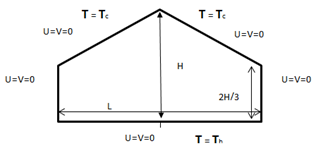
The configuration considered here is a 2D single-chapel greenhouse, heated from below (imposed temperature). The vertical walls are kept adiabatic while the roof is kept cold Figure 1. The greenhouse is filled with air assumed to be an incompressible Newtonian fluid with Pr = 0.71. The variation in density is subject to the Boussinesq approximation.
Figure 1. Geometry and boundary conditions
The LBM method is a relatively recent method for reproducing the behavior of complex fluids and has aroused the interest of many researchers in digital physics. It is an interesting alternative, which makes it possible to simulate complex physical phenomena by macroscopic nature. Its significant parallelization capacity also makes it attractive in order to perform rapid simulations on parallel equipment. The Boltzmann method on the network is an alternative method of simulating fluid flows. Unlike the traditional approach based on NAVIER-STOKES equations, the method consists in discretizing the Boltzmann equation, corresponding to a statistical modeling of the dynamics of the particles constituting the fluid. The Boltzmann method on the network has good advantages over conventional methods, in particular for the treatment of the domains of simulation complexes.
3.1 Dynamic model
The distribution function of a particle fi(x,t) is the probability of finding a particle at the site x at a time t, moving in a direction i at a velocity of:
$e_{i}=\frac{\Delta x_{i}}{\Delta t}$
The distribution function of the lattice Boltzmann equation for a particle is given by:
$\partial f_{i}(x, t)+e_{i} \nabla f_{i}(x, t)=\Omega_{i}(f)$ (1)
Such as $\Omega i(f)$ represents the rate of change of a particle after a collision. By adopting the simple approximation of relaxation time BGK, we obtain the linearized form of the collision operator:
$\Omega_{i}(f)=\frac{1}{\tau}\left(f_{i}^{e q}(x, t)-f_{i}(x, t)\right)$ (2)
where, τ is the relaxation time, and $f_{i}^{e q}(x, t)$ the distribution function at equilibrium. The introduction of the collision operator formula in Eq. (1), leads to the lattice equation BGK (model LBGK):
$\partial f_{i}(x, t)+e_{i} \nabla f_{i}(x, t)=\frac{1}{\tau}\left(f_{i}^{e q}(x, t)-f_{i}(x, t)\right)$ (3)
The integration of this equation with respect to time gives rise to the simplified form of the lattice Boltzmann equation:
$\begin{aligned} f_{i}\left(x+e_{i} \Delta t, t+\Delta t\right)=& f_{i}(x, t)+\\ & \frac{\Delta t}{\tau}\left(f_{i}^{e q}(x, t)-f_{i}(x, t)\right) \end{aligned}$ (4)
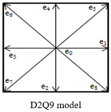
The LB method is thus entirely defined by choice of the equilibrium distribution function [29], which is relative to the chosen model. For the square model FHP denoted by D2Q9:
The equilibrium distribution function is explained as follows:
$f_{i}^{e q}=\omega_{i} \rho\left[1+3 \frac{e_{i} u}{c^{2}}+\frac{9}{2} \frac{\left(e_{i} u\right)^{2}}{c^{4}}-\frac{3}{2} \frac{u u}{c^{4}}\right]$ (5)
The macroscopic hydrodynamic quantities are determined through moments in phase space:
$\rho(x, t)=\sum_{i} f_{i}(x, t)$ (6)
$\rho u(x, t)=\sum_{i} e_{i} f_{i}(x, t)$ (7)
Chapman-Enskog's procedure allows us to retrieve Navier-Stokes' equations. Viscosity is related to relaxation time by the following formula:
$v=\left(\tau_{v}-\frac{1}{2}\right) c_{s}^{2} \delta t$ (8)
3.2 Thermic model
For the calculation of the temperature field, a second equation LBGK is taken into account:
$g_{i}\left(x+e_{i}, t+\Delta t\right)=g_{i}(x, t)+\frac{1}{\tau_{h}}\left(g_{i}(x, t)-g_{i}^{e q}(x, t)\right)$ (9)
As gi represents the function of energy distribution and τT the dimensionless time of relaxation, relating to the temperature field. The macroscopic temperature is thus calculated by:
$T_{i}=\sum_{i} g$ (10)
Thermal diffusivity is related to the relaxation time through
$\alpha=\frac{1}{3}\left(\tau_{T}-\frac{1}{2}\right) c^{2} \delta t$ (11)
The calculation code has been validated on a problem of natural convection of air confined in a square cavity with vertical walls that are differentially heated and with adiabatic horizontal walls. Our results were compared with those obtained by De Vahl Davis (1983). The latter addressed the same problem by adopting the finite difference method with the vortices-streamline function formulation (see Table 1).
However, experimental validation remains the essential element for testing our used digital models and the reliability of the boundary conditions chosen. The numerically determined air motions are consistent with [30, 31], and a good agreement between numerical and experimental results is found.
Table 1. The values of Raleigh and Nusselt number
|
|
Nu avg Hot Wall |
|
|
|
Present Work |
De Vahl Davis |
|
Ra =103 |
1.11 |
1.12 |
|
Ra =104 |
2.248 |
2.243 |
|
Ra =106 |
4.55 |
4.52 |
In this study, the streamlines, the isotherms, as well as the different profiles, will be presented for a single-capacity greenhouse heated by the ground (imposed temperature).
Streamlines and isotherms for form ratios, with A=L/H=2 (L=8m and L=4m).
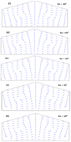
5.1 Velocity fields and contours
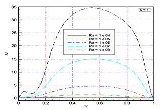
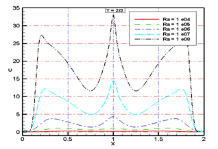
Two configurations shown in Figures 2 and 3, the velocity vectors clearly show the air movement inside the greenhouse, with two counter-rotating loops occupying the entire volume. Critical speed gradients are clearly observed at the level of the side walls, the ground, the roof, and in the center of the greenhouse (coincidence zone of the two rollers). The same observations are reported [32], who has studied natural turbulent convection by PIV, from which they have shown that in horizontal boundary layers (except in the inter-roll zones) and at roll intersections, velocities are the highest. On the other hand, low velocities are recorded in the center and corners of the cells; the same observations are reported [30, 31]. Figure 5 shows the vertical profile of the velocities, we notice that they cancel each other out at ground and roof level, on the other hand in the center, where they take maximum values, the difference that we can observe that the highest velocity is that of the high Ra number. Figure 6 shows the distribution of velocity curves at the horizontal level of the greenhouse at 2/3 H height. There is a symmetry by contribution to the center of the greenhouse. In addition, the high speeds are close to the vertical walls and in the center of the greenhouse.
Figure 2. Streamlines for different Raleigh numbers
Figures 3. Velocity vectors for different Raleigh numbers
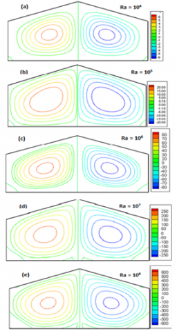
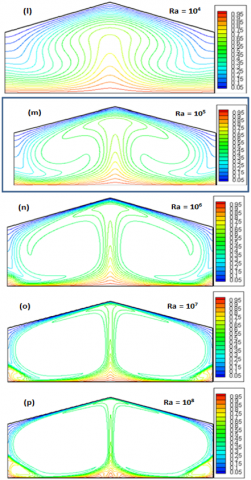
5.2 Isotherms
Figure 4 gives an example of the air movement inside the greenhouse, in this work and in related references it was observed that the temperature distribution inside the greenhouse follows circular current lines; they reached the maximal value towards the center. Which is identical to that reported by Awbi, Hatton [30, 33] who studied natural convection in a horizontal panel, and room respectively heated from the bottom, they came to the same conclusions.
The temperature distribution shape is different from figure to another due to the Rayleigh numbers as well as the air movement inside the greenhouse.
When calculations are carried out starting with low Rayleigh numbers the flow regime is as we can expect almost conductive which implies that the fluids circulation is not intense enough, as well as the Rayleigh number's increase the natural convection effect manifest. More and more when the Ra numbers is greater than 106 Figures 4 (o, p) it was observed the appearance of two small cells in the greenhouse lower corners.
Figure 4. Isotherms for different Raleigh numbers
5.3 Temperature profile
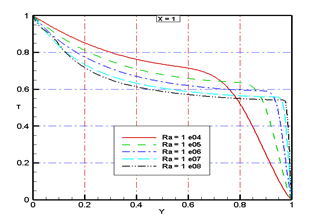
5.3.1 Vertical
The vertical temperature profile shown in Figure 7 follows the air distribution. It is characterized by strong thermal gradients near the ground and the roof, but the air temperature remains almost constant throughout the entire volume of the greenhouse, reaching the same conclusion [34]. On a reduced scale, they observed strong temperature gradients in the thin layers next to the ground and the roof, whereas inside the greenhouse, the temperature is stable [29], who investigated natural convection, observed the same phenomenon.
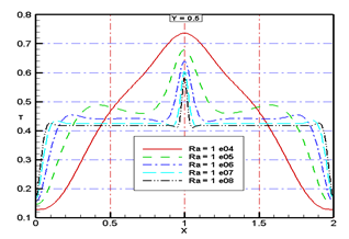
5.3.2 Horizontal
Figure 8 shows the h temperature profile. We can see that this profile is symmetrical in relation to the center of the greenhouse, the high temperatures are in the vicinity of the vertical walls and in the center of the greenhouse because of the air movement in these areas.
Figure 5. Air velocity, vertical distribution in the center of the greenhouse
Figure 6. Air velocity, horizontal distribution ($\frac{2}{3} \mathrm{H}$) above the ground
Figure 7. Air temperature, vertical distribution in the center of the greenhouse
Figure 8. Air temperature, horizontal distribution ($\frac{2}{3} \mathrm{H}$) above the ground
This paper is a modest contribution to the ongoing discussions about the behavior of the air inside the greenhouse. The author´s attention was focused a development of mathematical model as well as Particular attention is paid to using the lattice Boltzmann method. that allowed us to determine the spatial and temporal distributions of temperature velocity and isotherms across the study field.
We have also considered the consequences of buoyancy forces inside greenhouses air circulation and temperature distribution. The air circulation is characterized by two counter-rotating cells with high speeds along the sidewalls, roof, floor, and in the center of the greenhouse (coincidence zone of the two rollers). Low speeds, on the other hand, are recorded in the center and corners of the cells.
The overall results are summarized as following:
The evolution of the temperature in the greenhouse keeps the same pace for the different numbers of Raleigh also a peak in the plane which separates the two counter-rotating cells, strong thermal gradients develop in the boundary layers near the ground and the roof.
The temperature difference between the ground and the center of the greenhouse is greater than that between the roof and the center, this can be explained by the large difference in inertia between the ground and the wall.
The method is an effective way to improve eventually improve the thermal design of the greenhouses as well as the positioning of the air conditioning systems.
The analysis and simulation eventually indicate that improve the thermal greenhouses design as well as the positioning of the air conditioning systems.
The simulation results match the calculations are in good agreement with earlier mentioned documents.
|
fi |
Single particle distribution function for density |
|
gi |
Single particle distribution function for temperature |
|
fieq |
equilibrium distribution functions for dynamic |
|
gieq |
equilibrium distribution functions for thermal field |
|
ei |
Discrete Lattice speed |
|
wi |
Weights for the particle equilibrium distribution function |
|
$\rho$ |
Density of flow (Kg/m3) |
|
T |
Temperature (K) |
|
$\tau_{V}$ |
Single particle relaxation times for density |
|
$\tau_{T}$ |
Single particle relaxation times for temperature |
|
α |
Thermal diffusivity (m2/S) |
|
n |
Kinematic viscosity (m2/S) |
[1] De Gelder, A., Dieleman, J.A., Bot, G.P.A., Marcelis, L.F.M. (2012). An overview of climate and crop yield in closed greenhouses. Journal of Horticultural Science and Biotechnology, 87(3): 193-202. http://dx.doi.org/10.1080/14620316.2012.11512852
[2] Grisey, A., Grasselly, D., Rosso, L., D'Amaral, F., Melamedoff, S. (2011). Using heat exchangers to cool and heat a closed tomato greenhouse: Application in the south of France. Acta Horticulturae (ISHS), 893: 405-411. https://doi.org/10.17660/ActaHortic.2011.893.38
[3] Vadiee, A., Martin, V. (2014). Energy management strategies for commercial greenhouses. Applied Energy, 114: 880-888. https://doi.org/10.1016/j.apenergy.2013.08.089
[4] De Dios, V., Roy, R., Ferrio, J., Alday, J.P., Landais, D.G., Milcu, A. (2015). Processes driving nocturnal transpiration and implications for estimating land evapotranspiration. Scientific Reports, 5: 10975-10975. https://doi.org/10.1038/srep10975
[5] Johnson, H.B., Polley, H.W., Whitis, R.P. (2000). Elongated chambers for field studies across atmospheric CO2 gradients. Functional Ecology, 14: 388-396. https://doi.org/10.1046/j.1365-2435.2000.00435.x
[6] Lawton, J.H. (1996). The ecotron facility at silwood park: The value of “big bottle” experiments. Ecology, 77(3): 665-669. https://doi.org/10.2307/2265488
[7] Arfaoui, N., Bouadila, S., Guizani, A. (2017). A highly efficient solution of off-sunshine solar air heating using two packedbed soflatent storage energy. Solar Energy, 155: 1243-1253. https://doi.org/10.1016/j.solener.2017.07.075
[8] Lazaar, M., Kooli, S., Hazarni, M., Farhat, A., Belghith, A. (2004). Use of solar energy for the agricultural greenhouses autonomous conditioning. Desalination, 168: 169-175. https://doi.org/10.1016/j.desal.2004.06.183
[9] Harjunowibowo, D., Cuce, E., Omer, S.A., Riffat, S.B. (2016). Recent passive technologies of green-house systems-review. 15 the International Conference on Sustainable Energy Technologies SET2016, 19th -22nd National University of Singapore, Singapore of July 2016.
[10] Kinan, A., Che Sidika, N.A. (2016). Experimental studies on small scale of solar updraft power plant. Journal of Advanced Research Design, 22(15): 1-12.
[11] Boulard, T., Wang, S. (2000). Greenhouse crop transpiration simulation from external climate conditions. Agricultural and Forest Meteorology, 100(1): 25-34. https://doi.org/10.1016/S0168-1923(99)00082-9
[12] Rabehi, A., Guermoui, M., Djemoui, L. (2018). Hybrid models for global solar radiation prediction: Caseofstudy. International Journal of Ambient Energy, 41(1): 31-40. https://doi.org/10.1080/01430750.2018.1443498
[13] Khelifi, R., Mawloud, G., Abdelaziz, R., Djemoui, L. (2018). Multi-step ahead forecasting of daily solar radiation components in saharan climate. International Journal of Ambient Energy, 41(6): 707-715. https://doi.org/10.1080/01430750.2018.1490349
[14] Zaiani, .M, Djafer, D., Chouireb, F. (2017). New approach to establish a clear sky global solar irradiance model. International Journal of Renewable Energy Research, 7(3): 1454-1462.
[15] Baille, A., Mermier, M. (1980). Utilisation des eaux de rejet en agriculture, I. Modifications microclimatiques dues au chauffage du sol par tuyaux enterrées, en plein champ. Agricultural and Forest Meteorology, 22: 23-34. https://doi.org/10.1615/ICHMT.2004.CHT-04.260
[16] Makhlouf, S. (1988). Expérimentation et modélisation d'une serre solaire à air avec stockage par chaleur latente assisté par pompe à chaleur de déshumidification. Thèse de Doctorat Université de Nice (1988).
[17] Boulard, T., Razafinjohany, E., Baille, A. (1989). Heat and water vapour transfer in a greenhouse witan anderground heat storage system part I. Experimental results. Agricultural and Forest Meteorology, 45: 175-184. http://dx.doi.org/10.1016/0168-1923(89)90042-7
[18] Tadj, N., Mohammed, A.N., Draoui, B., Kittas, C. (2017). CFD simulation of heating greenhouse using a perforated polyethylene ducts. International Journal of Engineering Systems Modelling and Simulation (IJESMS), 9(1). https://doi.org/10.1504/IJESMS.2017.081730
[19] Draoui, B. (1994). Caractérisation et analyse du comportement thermohydrique d'une serre horticole: identification in-situ des paramètres d'un modèle dynamique. Thèse de Doctorat en Energétique, Université de Nice Sophia Antipolis (1994).
[20] Kittas, C., Draoui, B., Boulard, T. (1995). Quantification du taux d’aération d'une serres à ouvrant continu en toiture. Agricultural and Forest Meteorology, 77(1-2): 95-111. https://doi.org/10.1016/0168-1923(95)02232-M
[21] BOULARD, T. (1996). CaracteHrisation et mode Hlisation du climat des serres: application ala climatisation estivale. [Characterisation and modelling of the climate of the greenhouses: Application to summer air-conditioning.]. These de l'ENSA de Montpellier, 1996. https://www.theses.fr/1996ENSA0001
[22] De villèle, O. (1974). Besoins en eau des cultures sous serre - essai de conduite des arrosa ges en fonction de l'ensoleillement. Acta Hortic., 35: 123-135 https://doi.org/10.17660/ActaHortic.1974.35.16
[23] Boulard, T., Baille, A., Le Gall, F. (1990). Etude de différentes méthodes de refroidissement sur le climat et la transpiration de tomates de serre. Elsiver/INRA, 543-553.
[24] Boulard, T., Jemaa, R. (1993). Greenhouse tomato crops transpiration, application to irrigation control. Acta Horticulture, 335: 381-387. https://doi.org/10.17660/ActaHortic.1993.335.46
[25] Boulard, T., Draoui, B., Neirac, F. (1993). Analyse du bilan thermohydrique d'une serre horticole. Application à la maîtrise du microclimat. Colloque Annuel de la Société Française des thermiciens, pp. 632-647.
[26] Nara, M. (1979). Studies on air distribution in farm buildings - Two dimensional numerical and experiment. Journal of the Society of Agricultural Structures, 9(2): 18-25. https://doi.org/10.11449/sasj1971.9.2_18
[27] Lamrani, M.A. (1997). Caractérisation et modélisation de la convection naturelle laminaire et turbulente à l’intérieur d'une serre. Thèse de Doctorat. Université d’Ibnou zohr (Agadir) (1997).
[28] Boular, T., Haxaire, R., Lamrani, A., Roy, J.C., Jafrin, A. (1999). Characterization and modelling of the air fluxes induced by natural ventilation in a greenhouse. Journal of Agricultural Engineering Research, 74(2): 135-144. https://doi.org/10.1006/jaer.1999.0442
[29] Dardi, O., McCloskey, J. (1998). Lattice Boltzmann scheme with real numbered solid density for the simulation of flow in porous media. Phys. Rev. E, 57: 4834-4837. https://doi.org/10.1103/PhysRevE.57.4834
[30] Pretot, S., Zeghmati, B., Le Palec, G. (2000). Theoretical and experimental study of naturalconvection on a horizontal plate. Applied Thermal Engineering, 20(10): 873-891. https://doi.org/10.1016/S1359-4311(99)00067-8
[31] Boulard, T., Wang, S. (2002). Experimental and numerical studies on the heterogeneity of crop transpiration in a plastic tunnel. Computers and Electronics in Agriculture, 34(1-3): 173-190. https://doi.org/10.1016/S0168-1699(01)00186-7
[32] Benkhlifa, A., Penot, F. (2006). la convection de Rayleigh-Bénard turbulente: Caractérisation dynamique par PIV. Revue des Energies Renouvelables, 9(4): 341-354.
[33] Awbi, H.B., Hatton, A. (1999). Natural convection from heated room surfaces. Energy and Buildings, 30: 233-244. https://doi.org/10.1016/S0378-7788(99)00004-3
[34] Boulard, T., Lamrani, A., Roy, J.C., Jafrin, A., Bouirden, L. (1998). Natural ventilation by thermal effect in one-half scale model mono-span greenhouse. American Society of Agricultural Engineers, 41(3): 773-781. https://doi.org/10.13031/2013.17214