Hadeel Qays Hashim* | Khamis Naba Sayl
© 2020 IIETA. This article is published by IIETA and is licensed under the CC BY 4.0 license (http://creativecommons.org/licenses/by/4.0/).
OPEN ACCESS
Runoff estimation in a watershed is very important for efficient management of scarce water resources. Soil information is essential information for runoff estimation. Data collecting and determination of soil textural classification for large territory using the traditional method, i.e. laboratory testing is time-consuming and costly. Therefore, this study suggested a model based on the combination of Radial Basis Neural Network (RBNN) model, Geographic Information System (GIS), Remote Sensing (RS) and field data to create a digital soil map. This model was studied as a case study in western Iraq, and it was tested using performance parameters. The findings of this model were further confirmed using the hydrological soil group developed by the United States Geological Survey (USGS). The adopted model has been successful in predicting the spatial distribution of clay soil, followed by both silt and sand. It was also noted that the Root Mean Square Error (RMSE) for clay, silt and sand is 4.2 percent, 9.5 percent and 11.0 percent respectively, while the highest value was for the coefficient of clay soil correlation (0.749). Furthermore, there are only four samples out of 25 that have minor variations in the estimated and measured soil texture category defined by USGS. The methodology adopted in this study is therefore well practical for soil classification. Additionally, a broad scale will produce high-quality runoff measurement.
artificial neural network, hydrological soil group, Remote Sensing (RS), Geographic Information System (GIS), runoff depth, Soil Conservation Service-Curve Number (SCS-CN)
For both arid and semi-arid regions one of the most significant natural resources is freshwater. Nevertheless, according to the paper [1], only 1 percent of the 2.5 percent extensive freshwater is obtainable for human use. One of the promising alternatives for freshwater is water that is stored and used especially in the arid and semi-arid area from the surface runoff. The west desert of Iraq is categorized as an arid region and it suffers from water scarcity [2]. Surface runoff has the potential to be available and safe to human needs. Precise measurement of surface runoff and its volume plays a key role in the management of the watershed in arid and semi-arid regions. Nonetheless, large scale runoff estimation was a difficult task. Therefore, more work is needed.
Recently, uncalibrated distribution runoff-rainfall models were obtained when runoff data are unachievable to simulate catchment rainfall-runoff response in semi-arid regions [3-5]. These models all have drawbacks. They need several input factors that reflect different catchment characteristics, and they also do not completely produce spatially distributed predictions of runoff values. This is because data collection for large catchment area is complicated and time-consuming. However, optimized runoff-rainfall model was successfully applied to achieve practical runoff simulation where such data is available in these regions [6]. The construction and implementation of a large-scale optimized rainfall-runoff model is difficult due to the lack of detailed field data. The rate of runoff to rainfall relies on the texture of the soil which is known to be the key parameter influencing the catchment runoff. Soil texture is therefore an important factor in terms of the stability and the surface runoff capacity [1].
The Soil Conservation Service (SCS) method is the most widely used in hydrology to predict runoff from rainfall from a satisfied rainfall event [1]. GIS is capable of handling various spatial data needed for modeling and can be used as a tool in distributed hydrological modeling. GIS spatially distributed modeling approach applying the curve number (CN) framework has been used in several studies [7-14]. This modeling process depends on which CN is given. CN is a derivative of land use/cover and texture of soils. Many hydrological models use CN as input to estimate storm runoff, such as Environmental Policy Integrated Climate (EPIC) [15], Soil and Water Assessment Tool (SWAT) [16] and Agricultural Non-Point Source Pollution (AGNPS) [17].
Unadventurously, the determination of the soil texture has been checked in the laboratory, and this method is expensive and time-consuming. RS is one of the most available approaches and the best solutions could provide the ability to extend obtainable soil survey data sets. Indeed, remote sensing is a very significant technique focused on different ranges of the electromagnetic spectrum to predict soil characteristics on various spatial scales [18]. The chemical and physical properties of materials define their spectral reflectance and emittance spectra, which can be used to identify them. Spectral reflectance refers the ratio of radiant energy reflected to the incident energy on a body [19].
Many studies have found that some textual classification of soil can be easily determined based on specific absorption characteristics on a local and laboratory scale [20-23]. The connection between laboratory analysis and image data of French Satellite for observation of Earth (SPOT), Landsat TM, and airborne spectroscopy was shown by Proctor et al. to regulate differences in soil texture class [24]. Five curves formed by Stoner and Baumgardner describe the relationship between spectral reflection and classification of soil that is based on texture and grain size [25]. The image dimension with band 2 and band 8 of Advance Spaceborne Thermal Emission and Reflection (ASTER) was used to estimate the soil texture groups [22]. ASTER`s short wave with band 5 and band 6 can detect clay soil, sandy soil and dark clay soil [23, 26].
The reflectance of the soil is very complex. Consequently, estimating the soil properties based on the physical model is a difficult task [27]. Therefore, we need a method that is able to reveal the complex relationships between reflectance and soil properties.
The current research provides an intelligible method for predicting the surface runoff using integrated GIS and RS data based on soil textural classification. The main aim of this study is to generate a digital soil map based on the spectral reflectance bands with laboratory testing of soil data using the Artificial Neural Network (ANN) model known as RBNN hybrid with GIS model. This map is a base of the hydrological model, which uses GIS to implement the CN method. The current study has proposed a methodology that is of paramount importance to obtain data which are almost minimal and hard to collect. The suggested method has been tested to investigate a field of research in Iraq, particularly in the west desert.
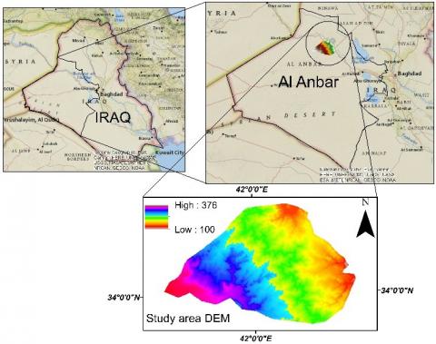
The main study has been implemented in Al-Anbar province, near Haditha city, in the west part of Euphrates river between 33º 50' 0" to 34º 20' 0" north and 41º 40' 0" to 42º 20' 0" east and has an area 1953.1 km2 Figure 1. It is surrounded to the north by the city of Ana, to the southwest by the Horan valley, to the west by the Euphrates river. A number of valleys are included in the study area: Al-Fahami, Hijlan and Zgdan and with an area 1020, 447.8, and 485.3 km2, respectively. The climate of the study area is hot-dry in the summer and fairly cold in the winter. The average temperature fluctuation is about 36ºC. As a result of this variability, the land surface can be broken into fragments and points. As for evaporations, its amount is (3200 mm) per year. All the precipitation comes during the winter and spring months. The research area average annual rainfall is estimated to be 115mm using monthly data for the years between (1989-2019) Iraqi metrological seismological organizations. The present dry environment can cause mechanical surface interruption. The lowest and highest elevations of research area scales, respectively, are 117 and 338 m above sea level.
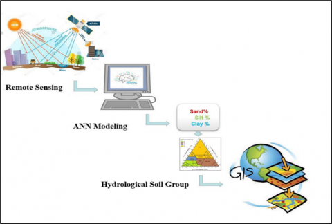
The following approach consists of several steps in the selection, preparation, and modeling of data to achieve the purpose of this study. The satellite images of the study area from Landsat 8 in Jun 2019 are prepared. The main idea of the proposed methodology epitomized in Figure 2.
Figure 1. Study area location
Figure 2. Representation of methodology for the study
This methodology is represented in the following steps:
First step, the unsupervised classification performed after the image was corrected with WGS 84/UTM zone 38 projection. This categorization was done in order to collect the most important data required to attain the aims of the present research. This involves the process required to categorize pixels into a restricted number of data sets based on the importance of the data collected [28]. Each pixel has been rated in the various wavelength bands by its comparative reflectance. This process was conducted using ArcGIS software to detect and verify the foremost classes of soil texture in the field of study. Nonetheless, unsupervised classification can be used as pre-processing prior to acquire an impression of main classes [29]. When field data is lacking and the research area is very large, this approach is preferred. It is also acknowledged, however, that the unsupervised classification can be beneficial in the elaboration of the embryonic map for reconnaissance and soil survey, to identify places for soil samples. The findings of this process offer a good representation of certain classes and classified these classes based on the ranges of the image value, and also for surveying soil with a view to reducing the time and cost consumption.
Second step, sampling locations were selected in this step (120) based on the previous step. Where the places to cover the whole field of study area chosen and where all groups are included in the map. Using GPS, the sample point in this study was located. Whereas in the topsoil, the samples obtained by auger and depths were 20-40. Subsequently, laboratory testing is used to predict the texture of the soil for each sample using sieve analysis and hydrometer test.
Third step, using a Landsat 8 satellite image to evaluate each location's spectral reflection, these images are represented by nine bands, using ArcGIS 10.7., while two thermal bands have been reduced.
Fourth step, a sensitivity analysis was performed to define the complicity of the band-to-soil texture relationship as (clay%, silt%, sand%). Using the RBNN model, the spectral reflection and the percentages of soil textures were used as a database to create a mathematical model. There are three layers in this model that are input layer which is used for the network feeding feature matrix, the hidden layer where the base function result calculation is processed, and the linear output layer for the basic functions combined. This model is relying on the process of interpolation of a multivariate function and one of its characteristics is that the number of radial base functions within the hidden layer depends not on the size of the data collection but on the complexity of the data. Thus, as for the finding, the results of the neural network are incorporated into GIS to provide a soil map for the catchment. The results of this model have been evaluated using Root mean square error (RMSE), Normalized root mean square error (NRMSE), Mean absolute error (MAE), Normalized mean absolute error (NMAE), Minimum absolute error, Maximum absolute error, Correlation coefficient (r).
Fifth step, inside ArcGIS 10.7, the results of the model were modified with the spatial analyst model as a tool for producing a digital map for the study are of the hydrological soil group.
Final step, the key environmental factors associated with the rainfall-runoff process are used in the SCS method such as hydrological soil group, rainfall, land use/land cover and soil types to define the depth of runoff as defined in equations [30].
$Q=\frac{(p-0.2 S)^{2}}{(p+0.8 S)}$ (1)
$S=\frac{25400}{C N}-254$ (2)
where, Q represents direct runoff depth mm, p is the rainfall depth mm, S is the potential maximum retention after runoff begins mm, CN refers to a dimensionless runoff index defined based on HSG and land use.
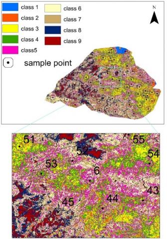
It was found that the unsupervised classification offers an appropriate and detailed description of certain sets. Therefore, these sets are graded depending only on the image value. Consequently, using the unsupervised classification can be a suitable method for constructing an embryonic map to assemble soil samples. This method would diminish task expenses and time. The selection of the soil sample position is carried out on the basis of certain parameters in order to avoid the errors associated with spectral reflectance and to perform accurate estimation of soil type. Figure 3 indicates the selected portion of the study area that carries out the unsupervised classification. In this figure there are nine classes, representing the land cover classes, each class is presumed to be a specific color. This figure shows the number and location of each sample where they were taken in various groups for laboratory research. There are 13 samples in and out of each class. There are 117 samples used with GPS tools to cover the entire study area. For each point, the spectral reflectance for nine bands was calculated using ArcGIS 10.7, and the results of the soil textures laboratory test were used as a database for developing a mathematical model using the RBNN model.
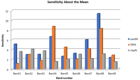
Sensitivity analysis was used to ensure the relationship of complexity between output as (sand%, silt%, clay%) and input data as spectral reflection. Figure 4 indicates the sensitivity of the clay, sand and silt to the bands. Clearly, Figure 4 shows that band 8, band 4, and band 7 comprise the highest degree of sensitivity to soil types, especially sand and silt, whereas band 2, band 3 and band 1 show a higher degree of the sensitivity of the clay. Additionally, the soil type and spectral reflection is very complicated where all bands contribute to the sense of soil type but in different weights. Hence, having all the bands in the Artificial Neural Network (ANN) model is important.
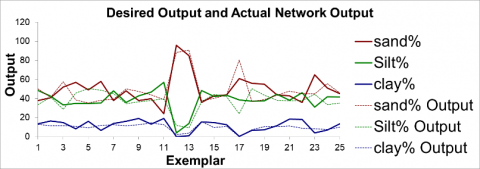
Estimated and actual ANN model values for 25 samples are shown in Figure 5. This figure indicates that the predicted clay values are more reliable than sand and silt because there is a significant fluctuation between the actual and estimated value for sandy and silt soil. Indeed, due to the constant comprehensive performance of this model, the total expected value of the ANN production is 100%. To determine the modeling performance where Table 1 presents ANN performance for each soil type. Obviously, it can be assumed that there is a significant difference in the precision of the three types of soil estimation values. Among other types, the clay predictor has higher results in all output parameters where the lowest RMSE, NRMSE, MAE, NMAE and minimum, maximum Abs error are (4.237, 0.2047, 3.489, 0.1685, 0.47866 and 8.9533 respectively) while the highest correlation coefficient is (r = 0.749). As seen in Figure 5, some fluctuation in outcomes can be shown by comparing sand and silt accuracies. Based on NRMSE and NMAE, estimating the silt works more efficiently than estimating the sand.
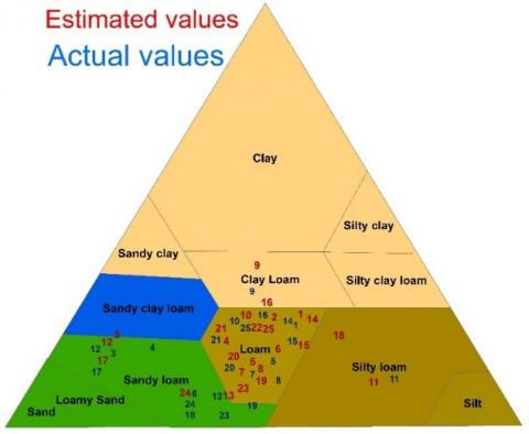
The results of estimated values of 25 samples obtained from the proposed model were evaluated by the USDA-developed hydrological soil groups, as is apparent in Figure 6. Nevertheless, the importance of this statistic in terms of soil texture indicates the real and expected values of the soil samples. Here we can analyze the model's actual overall performance in terms of hydrological soil group. The red (estimated) and blue (actual) numbers in the soil triangle provide the location of the test. Out of 25 samples in general, only 4 samples show minor differences in the estimated and calculated soil texture group. Notwithstanding the error in estimating soil texture of these samples but still in the same hydrological group that is the main target of this analysis. Ultimately, ANN's overall performance is quite superior to what was previously portrayed.
Figure 3. Unsupervised classification of the study area with samples location
Figure 4. Sensitivity of bands for clay, silt, sand
Table 1. Neural network models performance parameters for clay, silt and sand
|
Performance |
Sand% |
Silt% |
Clay% |
|
RMSE |
11.08087 |
9.503868 |
4.237794 |
|
NRMSE |
0.160592 |
0.140175 |
0.204724 |
|
MAE |
8.579605 |
8.07004 |
3.489235 |
|
NMAE |
0.124342 |
0.119027 |
0.168562 |
|
Min Abs Error |
0.068127 |
0.852735 |
0.47866 |
|
Max Abs Error |
20.11589 |
17.07785 |
8.953379 |
|
r |
0.732294 |
0.588528 |
0.749586 |
Figure 5. Estimated and actual values of sand, silt and clay for the tested samples
Figure 6. Estimated and actual points on the triangle of soil texture
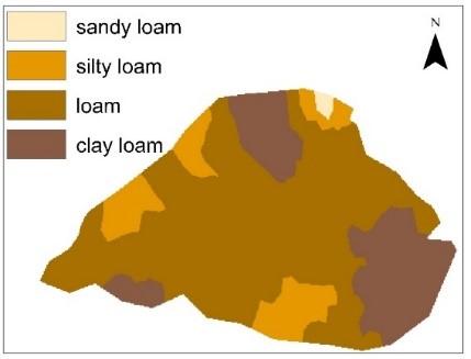
Figure 7. Digital soil map
Figure 8. Hydrological soil group map
The map of the estimated soil texture was developed for the study region by simulating the spectral reflectance of 1200 points at various locations in the ANN model (Figure 7). That figure represents this current study's final output. Then, the percentage of soil types listed according to the USDA hydrological soil classification. The results of the categorization calculated using GIS as a means of creating a digital map of the hydrological soil group by the spatial analyst model, as shown in Figure 8. This map shows the distribution of hydrological soil group over the study area which is a vital factor for investigation types of diversity.
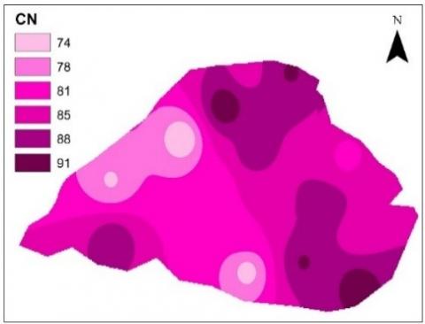
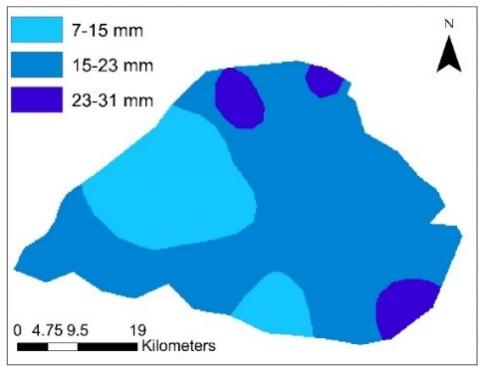
The runoff depth of the study area was calculated based on rainfall data from 1989 to 2019 from Iraqi meteorological and seismological organizations, and the study area weighted curve number, as shown in Figure 9. The maximum and minimum runoff distributed for the entire study region using the spatial analyst model within ArcGIS as Figure 10, according to the SCS curve number for the study area. As shown in Figure 10, the minimum and maximum values of runoff depth between 7 mm and 35 mm.
Figure 9. Curve Number map
Figure 10. Runoff depth map
Combining ANN with GIS, RS data, and data survey can be useful and helpful in developing methods that can be utilized to guess the runoff depth. Such approaches can provide the necessary information effectively as these analyzes are typically costly, time-consuming, and limited in recovering the temporal and spatial variability. In terms of the relationship between spectral reflection and soil texture, the soil class prediction has been developed. By merging an ANN model with GIS and RS data, this study can be considered as a proposed milestone and evaluated the method for predicting a digital soil map for a region. This technique was assessed on the basis of seven performance (one performance criteria) for clay, silt, and sand content were 4.2, 9.5, and 11.0 respectively. The highest correlation coefficient (0.749) was produced by the clay soils. Furthermore, there are only four samples out of 25 that have minor variations in the estimated and measured soil texture category defined by USG. However, all samples were located in the same hydrological soil group. Hence, the proposed methodology performs well for soil classification and can offer the information required for runoff depth estimates in an efficient manner. It is also fast and cost-effective.
[1] Jasrotia, A.S., Majhi, A., Singh, S. (2009). Water balance approach for rainwater harvesting using remote sensing and GIS techniques, Jammu Himalaya, India. Water Resources Management, 23(14): 3035-3055. https://doi.org/10.1007/s11269-009-9422-5
[2] Sulaiman, S., Kamel, A., Sayl, K., Alfadhel, M. (2019). Water resources management and sustainability over the Western desert of Iraq. Environmental Earth Sciences, 78: 495. https://doi.org/10.1007/s12665-019-8510-y
[3] Schulze, R.E. (1994). Hydrology and Agrohydrology: A Text to Accompany the ACRU 3.00 Agrohydrological Modelling System. Water Research Commission, Report TT69/95, Pretoria.
[4] Hughes, D.A. (1995). Monthly Rainfall–Runoff Models Applied to Arid and Semi‐Arid Catchments for Water Resource Estimation Purposes. Hydrological Science Journal, 40(6): 751-769. https://doi.org/10.1080/02626669509491463
[5] Anderson, N.J. (1997). Modelling the Sustainable Yield of Groundwater Resource in Riverbed Aquifers in Arid and Semi-arid Areas. MPhil to PhD Transfer Report. Department of Civil Engineering, University of London. London, England.
[6] Ye, W., Bates, B.C., Viney, N.R., Sivapalan, M., Jakeman, A.J. (1997). Performance of conceptual rainfall–runoff models in low yielding ephemeral catchments. Water Resources Research, 33(1): 153-166. https://doi.org/10.1029/96WR02840
[7] Thomas, A., Chingombe, W., Ayuk, J., Scheepers, T.A. (2009). Comprehensive Investigation of the KuilsEerste River Catchments Water Pollution and Development of a Catchment Sustainability Plan. Report to the Water Research Commission. December 2009. WRC Report No. 1692/1/10.
[8] Tsheko, R. (2006). Comparison between the united states soil conservation service (SCS) and the two models commonly used for estimating rainfall-runoff in south-eastern Botswana. Water SA, 32(1): 29-36. https://doi.org/10.4314/wsa.v32i1.5236
[9] Sharma, D., Kumar, V. (2002). Application of SCS model with GIS data base for estimation of runoff in an arid watershed. Journal of Soil and Water Conservation, 30(2): 141-145.
[10] Pandey, A., Sahu, A.K. (2004). Estimation of runoff using IRS-1 B LISS-II data. Indian Journal of Soil Conservation, 32(1): 58-60.
[11] Jain, M.K., Mishra, S.K., Singh, V.P. (2006). Evaluation of AMC- dependent SCS - CN - based models using watershed characteristics. Journal of Water Resources Management, 20(4): 531-555. https://doi.org/10.1007/s11269-006-3086-1
[12] Sayl, K.N., Muhammad, N.S., El-Shafie, A. (2017). Robust approach for optimal positioning and ranking potential rainwater harvesting structure (RWH): A case study of Iraq. Arabian Journal of Geosciences, 10(18): 413. https://doi.org/10.1007/s12517
[13] Sayl, K.N., Muhammad, N.S., El-Shafie, A. (2019). Identification of potential sites for runoff water harvesting. Proceedings of the Institution of Civil Engineers: Water Management, 172(3): 135-148. https://doi.org/10.1680/jwama.16.00109
[14] Sayl, K.N., Mohammed, A.S., Ahmed, A.D. (2020). GIS- based approach for rainwater harvesting site selection. IOP Conf. Series: Materials Science and Engineering, 737: 012246. https://doi.org/10.1088/1757-899X/737/1/012246
[15] Wang, X.Y., Williams, J.R., Gassman, P., Baffaut, C., Izaurralde, R.C., Jeong, J., Kiniry, J.R. (2012). Epic and Apex. Model use calibration, and validation. Transactions of the Asabe, 55(4): 1447-1462. https://doi.org/10.13031/2013.42253
[16] Neitsch, S., Arnold, J., Kiniry, J., Williams, J. (2011). Soil & Water Assessment Tool Theoretical Documentation Version 2009. Texas Water Resources Institute. Available electronically from http://hdl.handle.net/1969.1/128050, accessed on Mar. 1, 2020.
[17] Young, R., Onstad, C.A., Bosch, D.D., Anderson, W.P. (1987). AGNPS, Agricultural Non-Point-Source pollution model: A watershed analysis tool. Research Report.
[18] Lacoste, M., Minasny, B., McBratney, A., Michot, D., Viaud, V., Walter, C. (2014). High resolution 3D mapping of soil organic carbon in a heterogeneous agricultural landscape. Geoderma, 216: 296-311. https://doi.org/10.1016/j.geoderma.2013.07.002
[19] Sims, D., Gamon, J. (2002). Relationship between leaf pigment con- tent and spectral reflectance across a wide range species, leaf structures and development stages. Remote Sens. Environ., 81(2-3): 337-354. https://doi.org/10.1016/S0034-4257(02)00010-X
[20] Chang, C., Laird, D. (2002). Near-infrared reflectance spectroscopic analysis of soil C and N. Soil Science, 167(2): 110-116.
[21] Nanni, M., Demattê, J. (2006). Spectral reflectance methodology in comparison to traditional soil analysis. Soil Science Society of America, 70(2). https://doi.org/10.2136/sssaj2003.0285
[22] Apan, A., Kelly, R., Jensen, T., Butler, D., Strong, W., Basnet, B. (2002). Spectral discrimination and separability analysis of agricultural crops and soil attributes using ASTER imagery. In: 11th Australasian Remote Sensing and Photogrammetry Conference (ARSPC2002): Images to Information, 2-6 Sept 2002, Brisbane, Australia.
[23] Chabrillat, S., Goetz, A.F.H., Krosley, L., Olsen, H.W. (2002). Use of hyperspectral images in the identification and mapping of expansive clay soils and the role of spatial resolution. Remote Sensing of Environment, 82(2-3): 431-445. https://doi.org/10.1016/S0034-4257(02)00060-3
[24] Proctor, C.J., Baker, A., Barnes, W.L., Gilmour, M.A. (2000). A thousand-year speleothem proxy record of North Atlantic climate from Scotland. Climate Dynamics, 16: 815-820. https://doi.org/10.1007/s003820000077
[25] Stoner, E.R., Baumgardner, M.F. (1981). Characteristic variations in reflectance of surface soils. Soil Science Society of America Journal, 45(6): 1161. https://doi.org/10.1007/978-3-662-03978-6
[26] Breunig, F., Galvão, L. (2008). Detection of sandy soil surfaces using ASTER‐derived reflectance, emissivity and elevation data: potential for the identification of land degradation. International Journal of Remote Sensing, 29(6). https://doi.org/10.1080/01431160701851791
[27] Clark, R.N., Roush, T.L. (1984). Reflectance spectroscopy: Quantitative analysis techniques for remote sensing applications. Journal of Geophysical Research: Solid, 89(B7). https://doi.org/10.1029/JB089iB07p06329
[28] Jain, A.K. (1989). Fundamentals of Digital Image Processing. Prentice-Hall, Inc. Division of Simon and Schuster One Lake Street Upper Saddle River, NJ United States, 569 pages.
[29] Richards, J.A., Jia, X. (1999). Remote Sensing Digital Image Analysis. Springer-Verlag Berlin Heidelberg, New York. https://doi.org/10.1007/978-3-642-30062-2
[30] Maidment, D.R. (1992). Handbook of Hydrology. McGraw-Hill, New York, NY, USA.