A Novel Energy Consumption Prediction Model Combining Long Short-Term Memory (LSTM) and Fractional Differential Equations (FDLE)

Rapid urbanization, surging human population, and societal demand in the building sector are some of the factors driving the significant increase in household energy demand recently [1]. The global energy usage and the associated greenhouse gas emissions has been influenced by the increasing demand buildings [2]. It is important that buildings should be sustainable and energy-efficient and there is a need that utility companies, customers, and facility managers to understand the trends in building energy usage to improve energy efficiency. Scholars have developed interest in learning more about energy-saving and building energy efficiency [3, 4]. The study and examination of data through the use of AI-based techniques like machine learning (ML) have been eased with the advancement of Industry 4.0. Therefore, the prediction of the energy usage pattern in buildings has become necessary for better energy performance at the operation and maintenance phases of buildings.

The analysis of building energy patterns can be achieved using either the data-driven approach or the physics-based simulation approach [1]. The physics-based method requires the use of the whole building energy simulation tools like DOE-2 and Energy Plus. The users of these tools must provide the heat properties of the building components, such as walls, roofs, and windows, HVAC (heating, ventilation, and air conditioning) systems, thermal settings, internal loads of occupancy, building geometry, etc. but due to the lack of necessary data and time commitment, these techniques are not mostly useful for energy analysis throughout the operation and maintenance phases [5].

During energy analyses for various buildings, there are numerous problems associated with the physics-based approaches. Hence, data driven approaches were developed to mostly use past data to access building energy performance. The development of AI and IoT enables the use of this method to understand building energy usage patterns.  The use of this data-driven method requires access to open data. The use of ML for the estimation of the future pattern of energy usage of buildings has been proposed by many researchers. For instance, the use of ANN [6], decision trees (DT) [7], ANFIS [8], and SVM [9] for the prediction of building energy usage has been proposed. Artificial Neural Networks (ANN) are computational models inspired by the human brain, designed to recognize patterns and make predictions by learning from data through layers of interconnected nodes (neurons) [6]. Decision Trees (DT) are a type of supervised learning algorithm used for classification and regression tasks; they work by splitting the data into subsets based on feature values, forming a tree-like structure where each branch represents a decision rule [7]. Adaptive Neuro-Fuzzy Inference System (ANFIS) combines neural networks with fuzzy logic to model complex systems by learning from data and handling uncertainty through fuzzy rules, making it effective for control and prediction tasks [8]. Support Vector Machines (SVM) are powerful supervised learning algorithms used primarily for classification and regression; they work by finding the optimal hyperplane that separates data points of different classes in a high-dimensional space, often providing robust results even in cases where the data is not linearly separable [9].

The ever-increasing energy demand can be addressed by the use of energy efficient solutions, which can lower greenhouse gas emissions and improve energy security [2]. Batlle et al. (2020) considered the opportunities for energy reduction in buildings by creating energy baselines and energy performance indicators [10]. They observed that the educational facilities might save up to 9.6% of their annual energy costs by considering the developed energy performance indicators. The study also came up with a method for aiding decision-makers in putting urban greening policies into practice by statistically predicting the impact of green initiatives on building energy [11].

Based on the brief survey, The existing prediction models are either based on one or a small number of datasets for the training and testing processes which may impact the generalization of the model results. this is the first research gap of the current study. Besides, until now, only a few works have assessed the performance of models that uses different datasets to predict hourly building energy use which is can consider the second research gap. Therefore, this work intends to evaluate the applicability and efficacy of the DL model and a modified mathematical equation called fractional calculus in the prediction of future building energy usage using numerous experimental datasets. A new model called (LSTM-FDLE) was designed in this work for the forecasting of energy demand through the utilization of two emerging techniques - long short-term memory (LSTM) and fractional differential equations. The proposed LSTM-FDLE model was trained for accurate prediction of the collective active power generated by household appliances. It leverages the memory and sequential learning capabilities of LSTM to capture complex temporal intricacies and trends in energy usage data.

The research framework developed for this study is presented in this section; The method begins with a literature review and concludes with an assessment of the research's results. The literature review was aimed at looking for methods already in use for the prediction of household electric power usage. In the suggested methodology, there are 3 stages, and the output of each stage is used as the input for the next. Phase 1 is about the dataset reading while phase two is about pre-processing phase for preparing to train the LSTM- FDLE model. Finally, phase three is about model training and evaluation of the research achievements. Figure 1 depicts in detail the general methodology of the proposed LSTM- FDLE model. 

image003.png

Figure 1. Structural design of the suggested framework

3.1 The utilized dataset

The data utilized in this study called (Household Electric Power Consumption dataset) comprises 2,075,259 data points collected from a residence situated in Sceaux, France, spanning a period of 47 months, commencing in December 2006 and concluding in November 2010 [15]. These measurements were recorded at one-minute intervals. It's worth noting that this dataset might include some gaps, accounting for approximately 1.25% of the total entries. While the dataset contains all calendar timestamps, there are certain timestamps that do not have corresponding measurement values. These missing data points are identified by the lack of a value between two semicolons attribute separators.

The dataset will be used to develop a predictive model for the prediction of the global active power and household energy usage based on the explained parameters.

The EDA of the dataset is provided here [16, 17]; this includes 4 figures that further explained the dataset. There are numerous subplots in Figure 2, each depicting the mean resampled data for a specific variable on a monthly basis. Time (in months) is represented in the horizontal axis, while the average value of the variable is in the vertical axis. This figure improves understanding of the monthly trends in the data.

Like in Figure 2, the image in Figure 3 consists of multiple subplots but the data representation is on a daily basis. The mean of the resampled data for a specific variable is represented by each subplot; the duration is represented in the horizontal axis (in days) while the average value of the variable is in the vertical axis. This figure provides better understanding of the daily data variations and patterns.

Figure 4 is a representation of the data on an hourly basis where each subplot is a representation of the meaning of the resampled data for a given variable. The time in hours is plotted in the horizontal axis while the average value of the variable is in the vertical axis. This figure provides better understanding of the hourly changes and patterns in the data.

image004.jpg

Figure 2. The subplots for the monthly data trends and patterns

image005.jpg

Figure 3. Multiple subplots for the daily data variations and patterns

image006.jpg

Figure 4. Multiple subplots for the hourly changes and trends in the data

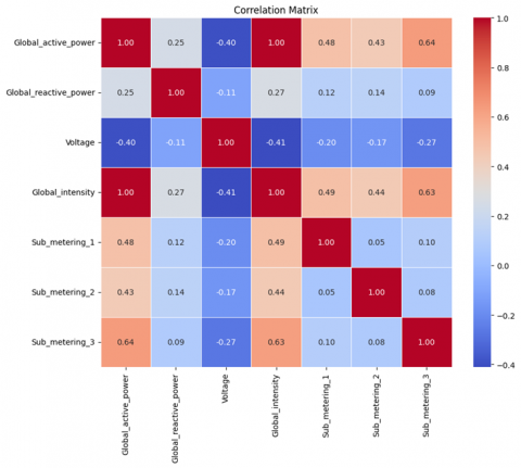
A correlation matrix heatmap is presented using a color map in Figure 5; it depicts the relationship between different parameters in the data. The strength and direction of the correlation is indicated by the values in the heatmap, where a positive value = positive correlation, negative value = negative correlation. Darker colors show strong correlations. This figure provides better view of the relationships between different data variables, as well as a knowledge of the trends, patterns, and correlations in the data.

image007.png

Figure 5. Correlations and dependencies between different data variables

3.2 Data pre-processing

The significance and novelty of using fractional differential equations (FDEs) in this context lie in their ability to model systems with memory and hereditary properties more accurately than classical differential equations. This approach allows for a more nuanced description of dynamic processes, particularly in cases where standard integer-order models fall short in capturing the complex behaviors of the system. Unlike traditional methods, FDEs provide greater flexibility in adjusting the model to account for non-local interactions and anomalous diffusion, which are common in many real-world applications, such as image processing or signal analysis. There are three important steps in the data preprocessing stage before the training phase of the developed LSTM- FDLE model; the first step is to removal of missing data from the dataset to ensure the completeness of the data for the training process and to avoid potential biases or inaccuracies caused by missing data. The next step is the data standardization step using the MinMaxScaler [18]. This process is mostly used to transform data into a common scale to improve effectiveness when using ML models [19]. The MinMaxScaler was used to scale the data to a specific range, mostly [0, 1] to ensure that the magnitude of all the features is similar. The final step is the preparation of the data as a time series by transforming it into a suitable format for the training process. His process requires the creation of lagged input and output variables that allows the network to learn patterns and dependencies over time. The completion of these preprocessing steps prepares the data for the training of the model on the prepared time series data.

Among the ML algorithms, RNNs have been the most used for sequential data modeling; they are used in many areas like speech recognition, time series data analysis, and natural language processing. The emphasis in this article is on the RNNs, especially LSTM networks and their usage for energy consumption prediction. Efficient energy management, demand projection, and resource allocation requires accurate energy consumption prediction. LSTM leverages the temporal connections and trends in energy usage data to predict the future energy usage pattern. A summary of RNNs and “LSTM” networks is presented here, focusing more on their foundations and their relevance in energy consumption prediction. The RNN is derived from differential equations and introduced from the general form of the state signal evolution equation. The special case of the state signal equation was also presented; the components involved in energy consumption prediction were also detailed.

An RNN was developed in this work using differential equations; the starting point is the definition of $ \overrightarrow{s}\left( \text{r} \right)$ as a d-dimensional state signal vector, as well as the analysis of the general nonlinear first-order non-homogeneous ODE; this will reveal the evolution of the state signal over time (r).

$\frac{\text{c}{\overrightarrow{s}}\left( \text{r} \right)}{\text{cr}}=\text{}{\overrightarrow{f}\left( \text{r} \right)+}\overrightarrow{\phi }$                          (6)

where, $\text{}{\overrightarrow{f}}\left( \text{r} \right)$ is a vector-valued function of time, where t is a positive real number. The vector ϕ is a constant with d dimensions. A common representation for$\text{ }\!\!~\!\!\text{}{\overrightarrow{f}}\left( \text{t} \right)$ is as follows:

$\overrightarrow{\mathrm{f}}(\mathrm{r})=\overrightarrow{\mathrm{h}}(\overrightarrow{\mathrm{s}}(\mathrm{r}), \overrightarrow{\mathrm{x}}(\mathrm{r}))$                            (7)

$\text{}{\overrightarrow{x}}\left( \text{r} \right)$ signifies the d-dimensional input signal vector, and the function  $\text{}{\overrightarrow{h}}\left( \text{}{\overrightarrow{s}}\left( \text{r} \right),\text{}{\overrightarrow{x}}\left( \text{r} \right) \right)$ takes vectors as arguments and yields a vector-valued result. The system that emerges from this formulation is encountered in a variety of scenarios within the fields of physics, chemistry, biology, and engineering.

$\frac{\text{c}{\overrightarrow{s}}\left( \text{r} \right)}{\text{ct}}=\text{}{\overrightarrow{h}}\left( \text{}{\overrightarrow{s}}\left( \text{r} \right),\text{}{\overrightarrow{x}}\left( \text{r} \right) \right)+\overrightarrow{\phi }$                          (8)

Finally, $\overrightarrow{\mathrm{x}}(\mathrm{r})$ is derived by gathering all the values of $x(\vec{i}, r)$ for all possible index components permutations into a column vector as seen in Eq. (8). An example of a particular scenario for $\text{}{\overrightarrow{f}}\left( \text{r} \right)$ in Eq. (9) is:

$\vec{f}(r)=\vec{a}(r)+\vec{d}(r)+\vec{c}(r)$                           (9)

The Additive Model will be analyzed to saturation as explained in Eq. (9). There are three elements of the model which are $  \overrightarrow{\mathrm{a}}(\mathrm{r}),~\vec{d}(\mathrm{r})$, and $\overrightarrow{\mathrm{c}}(\mathrm{r})$, and each element has its distinct definition.

$\begin{array}{*{35}{r}}  \text{}{\overrightarrow{a}}\left( \text{r} \right) & =\underset{\text{k}=0}{\overset{{{\text{K}}_{\text{s}}}-1}{\mathop \sum }}\,{{{\text{}{\overrightarrow{a}}}}_{\text{k}}}\left( \text{}{\overrightarrow{s}}\left( \text{r}-{{\text{ }\!\!\tau\!\!\text{ }}_{\text{s}}}\left( \text{k} \right) \right) \right)  \\ \end{array}$                  (10)

$\begin{array}{*{35}{r}}   \text{}{\overrightarrow{b}}\left( \text{r} \right) & \text{ }\!\!~\!\!\text{ }=\underset{\text{k}=0}{\overset{{{\text{K}}_{\text{r}}}-1}{\mathop \sum }}\,{{{\text{}{\overrightarrow{d}}}}_{\text{k}}}\left( \text{}{\overrightarrow{r}}\left( \text{t}-{{\text{ }\!\!\tau\!\!\text{ }}_{\text{r}}}\left( \text{k} \right) \right) \right)  \\ \end{array}$                  (11)

$\begin{array}{*{35}{r}}   \text{}{\overrightarrow{r}}\left( \text{r}-{{\text{ }\!\!\tau\!\!\text{ }}_{\text{r}}}\left( \text{k} \right) \right) & \text{ }\!\!~\!\!\text{ }=\text{G}\left( \text{}{\overrightarrow{s}}\left( \text{r}-{{\text{ }\!\!\tau\!\!\text{ }}_{\text{r}}}\left( \text{k} \right) \right) \right)  \\ \end{array}$                         (12)

$\begin{matrix}   \text{}{\overrightarrow{c}}\left( \text{r} \right) & \text{ }\!\!~\!\!\text{ }=\underset{\text{k}=0}{\overset{{{\text{K}}_{\text{x}}}-1}{\mathop \sum }}\,{{{\text{}{\overrightarrow{c}}}}_{\text{k}}}\left( \text{}{\overrightarrow{x}}\left( \text{r}-{{\text{ }\!\!\tau\!\!\text{ }}_{\text{x}}}\left( \text{k} \right) \right) \right)  \\ \end{matrix}$                           (13)

Using the given definitions, the system that resulted from replacing Eq. (10)-(13) into Eq. (6) and then incorporating the outcome into Eq. (1), can be expressed as follows:

$\frac{\overrightarrow{c s}(r)}{d t}=\sum_{k=0}^{K_s-1} \vec{a}_k\left(\vec{s}\left(r-\tau_s(k)\right)+\sum_{k=n}^{k_r-1} \vec{d}_k\left(\vec{r}\left(r-\tau_r(k)\right))+\sum_{k=0}^{K_k-1} \vec{c}_k\left(\vec{x}\left(r-\tau_x(k)\right))+\vec{\phi}\right.\right.\right.$                         (14)

$\begin{matrix}   \text{}{\overrightarrow{r}}\left( \text{r}-{{\text{ }\!\!\tau\!\!\text{ }}_{\text{r}}}\left( \text{k} \right) \right) & =\text{G}\left( \text{}{\overrightarrow{s}}\left( \text{r}-{{\text{ }\!\!\tau\!\!\text{ }}_{\text{r}}}\left( \text{k} \right) \right) \right)  \\   \end{matrix}$                              (15)

The first component: denoted as $\sum _{\text{k}=0}^{{{\text{K}}_{\text{s}}}-1}\vec{a}_{\text{k}}\left( \vec{s}\left( \text{r}-{{\text{ }\!\!\tau\!\!\text{ }}_{\text{s}}}\left( \text{k} \right) \right) \right)$, is a combination of up to ${{\text{K}}_{\text{s}}}$ functions. These functions are obtained by time-shifting the original functions, ${\vec{a}_{\text{k}}}\left( \vec{s}\left( \text{r} \right) \right)$, by specific delay time constants$\text{ }\!\!~\!\!\text{ }(\left. {{\text{ }\!\!\tau\!\!\text{ }}_{\text{s}}}\left( \text{k} \right) \right)$. It's worth noting that the term "analog" emphasizes that each ${\vec{a}_{\text{k}}}\left(\vec{s}\left( \text{r} \right) \right)$ depends on the state signal itself, rather than the readout signal, that is the transformed version of the state signal.

The second component: $\sum _{\text{k}=0}^{{{\text{K}}_{\text{r}}}-1}\vec{d}_{\text{k}}\left( \vec{r}\left( \text{r}-{{\text{ }\!\!\tau\!\!\text{ }}_{\text{r}}}\left( \text{k} \right) \right) \right)$, combines up to ${{\text{K}}_{\text{r}}}$ functions. These functions are generated by applying time shifts $\tau_{\mathrm{r}}(\mathrm{k})$ to the functions $\vec{d}_{\text{k}}\left( \vec{r}\left( \text{r} \right) \right)$. These functions originate from the readout signal, which is defined in Eq. (10) and represents a warped (potentially binary-valued) version of the state signal.

The third component: $\sum _{\text{k}=0}^{{{\text{K}}_{\text{x}}}-1}\vec{c}_{\text{k}}\left(\vec{x}\left( \text{r}-{{\text{ }\!\!\tau\!\!\text{ }}_{\text{x}}}\left( \text{k} \right) \right) \right)$, represents the external input; it is formed by aggregating up to ${{\text{K}}_{\text{x}}}$ functions, obtained by time-shifting ${{\text{ }\!\!\tau\!\!\text{ }}_{\text{x}}}\left( \text{k} \right)$ the functions $\vec{c}_{\text{k}}\left( \vec{x}\left( \text{r} \right) \right.$. These functions are associated with the input signal.

Consider a case where $\vec{a}_{\text{k}}\left( \vec{g}\left( \text{r}-{{\text{ }\!\!\tau\!\!\text{ }}_{\text{s}}}\left( \text{k} \right) \right) \right),\vec{d}_{\text{k}}\left(\vec{r}\left( \text{r}-{{\text{ }\!\!\tau\!\!\text{ }}_{\text{r}}}\left( \text{k} \right) \right) \right)$, and $\vec{c}_{\text{k}}\left(\vec{x}\left( \text{r}-{{\text{ }\!\!\tau\!\!\text{ }}_{\text{z}}}\left( \text{k} \right) \right) \right)$ are linear functions of $\vec{s},\vec{r}$, and $\vec{x}$, respectively; here, Eq. (9) is a nonlinear DDE with linear coefficients, and these coefficients are represented as matrices:

$\frac{\text{c}\vec{s}\left( \text{r} \right)}{\text{cr}}=\underset{\text{k}=0}{\overset{{{\text{K}}_{\text{s}}}-1}{\mathop \sum }}\,{{\text{A}}_{\text{k}}}\left(\vec{s}\left( \text{r}-{{\text{ }\!\!\tau\!\!\text{ }}_{\text{s}}}\left( \text{k} \right) \right) \right)+\underset{\text{k}=0}{\overset{{{\text{K}}_{\text{r}}}-1}{\mathop \sum }}\,{{\text{B}}_{\text{k}}}\left( \vec{r}\left( \text{r}-{{\text{ }\!\!\tau\!\!\text{ }}_{\text{r}}}\left( \text{k} \right) \right) \right)+\underset{\text{k}=0}{\overset{{{\text{K}}_{\text{x}}}-1}{\mathop \sum }}\,{{\text{C}}_{\text{k}}}\left( \vec{x}\left( \text{r}-{{\text{ }\!\!\tau\!\!\text{ }}_{\text{x}}}\left( \text{k} \right) \right) \right)+\vec{\phi }$                                      (16)

Moreover, in the case where the matrices ${{\text{A}}_{\text{k}}},{{\text{B}}_{\text{k}}}$, and ${{\text{C}}_{\text{k}}}$ are circulant or block circulant, the expression of the matrix-vector multiplication components given in Eq. (11) may be done as convolutions within the confines of the elements of $\text{}{\overrightarrow{s}},\text{}{\overrightarrow{r}},\text{}{\overrightarrow{x}}$, and $\overrightarrow{\phi }$. These convolutions are performed over each element indexed by $\text{}{\overrightarrow{i}}$:

$\frac{\text{cs}\left( \text{}{\overrightarrow{i}},\text{r} \right)}{\text{dr}}=\underset{\text{k}=0}{\overset{{{\text{K}}_{\text{n}}}-1}{\mathop \sum }}\,{{\text{a}}_{\text{k}}}\left( {\text{}{\overrightarrow{i}}} \right)\text{*s}\left( \text{}{\overrightarrow{i}},\text{r}-{{\text{ }\!\!\tau\!\!\text{ }}_{\text{s}}}\left( \text{k} \right) \right)+\underset{\text{k}=0}{\overset{{{\text{K}}_{\text{r}}}-1}{\mathop \sum }}\,{{\text{d}}_{\text{k}}}\left( {\text{}{\overrightarrow{i}}} \right)\text{*r}\left( \text{}{\overrightarrow{i}},\text{r}-{{\text{ }\!\!\tau\!\!\text{ }}_{\text{r}}}\left( \text{k} \right) \right)+\underset{\text{k}=0}{\overset{{{\text{K}}_{\text{z}}}-1}{\mathop \sum }}\,{{\text{c}}_{\text{k}}}\left( {\text{}{\overrightarrow{i}}} \right)\text{*x}\left( \text{}{\overrightarrow{i}},\text{r}-{{\text{ }\!\!\tau\!\!\text{ }}_{\text{z}}}\left( \text{k} \right) \right)+\phi \left( {\text{}{\overrightarrow{i}}} \right)$                         (17)

It is important to note that previous research has established a link between a nonlinear dynamical system, as defined in Eq. (14), and the extension of a specific type of neural network. This connection was demonstrated when the functions ${{\text{}{\overrightarrow{a}}}_{\text{k}}}\left( \text{}{\overrightarrow{s}}\left( \text{r} \right) \right),{{\text{}{\overrightarrow{d}}}_{\text{k}}}\left( \text{}{\overrightarrow{r}}\left( \text{r} \right) \right)$, and ${{\text{}{\overrightarrow{c}}}_{\text{k}}}\left( \text{}{\overrightarrow{x}}\left( \text{r} \right) \right)$ were linear operators in Eq. (16), resulting in the Continuous Hopfield Network as a specialized case. A closely related version, described in Eq. (17), which further limits these operators to be convolutional, was found to incorporate the Cellular Neural Network.

Applying the simplifications:

$\left. \begin{array}{*{35}{l}}   {{\text{K}}_{\text{s}}} & =1  \\   {{\text{ }\!\!\tau\!\!\text{ }}_{\text{s}}}\left( 0 \right) & =0  \\   {{\text{A}}_{0}} & =\text{A}  \\   {{\text{K}}_{\text{r}}} & =1  \\   {{\text{ }\!\!\tau\!\!\text{ }}_{\text{r}}}\left( 0 \right) & ={{\text{ }\!\!\tau\!\!\text{ }}_{0}}  \\   {{\text{B}}_{0}} & =\text{B}  \\   {{\text{K}}_{\text{x}}} & =1  \\   {{\text{ }\!\!\tau\!\!\text{ }}_{\text{x}}}\left( 0 \right) & =0  \\   {{\text{C}}_{0}} & =\text{C}  \\  \end{array} \right\}$                             (18)

(Although some of these constraints will be relaxed later), incorporating them into Eq. (16) transforms it into:

$\frac{\text{c}{\overrightarrow{s}}\left( \text{r} \right)}{\text{cr}}=\text{A}{\overrightarrow{s}}\left( \text{r} \right)+\text{B}{\overrightarrow{r}}\left( \text{r}-{{\text{ }\!\!\tau\!\!\text{ }}_{0}} \right)+\text{C}{\overrightarrow{x}}\left( \text{r} \right)+\overrightarrow{\phi }$                             (19)

Eqs. (16), (17), and (19) are examples of nonlinear first-order non-homogeneous DDEs. To solve these equations, as well as any other versions of Eq. (1), a common numerical method is to discretize them in time. This entails computing the values of both the timestamp input and state signals, continuing this process for the needed total duration. This results in numerical integration.

$\begin{array}{*{35}{r}}   \text{r} & \text{ }\!\!~\!\!\text{ }=\text{n }\!\!\Delta\!\!\text{ T }\!\!~\!\!\text{ }\left( 15 \right)  \\   \frac{\text{c}{\overrightarrow{g}}\left( \text{r} \right)}{\text{dr}} & \text{ }\!\!~\!\!\text{ }\approx \frac{\text{}{\overrightarrow{g}}\left( \text{n }\!\!\Delta\!\!\text{ T}+\text{ }\!\!\Delta\!\!\text{ T} \right)-\text{}{\overrightarrow{g}}\left( \text{n }\!\!\Delta\!\!\text{ T} \right)}{\text{ }\!\!\Delta\!\!\text{ T}}  \\ \end{array}$                               (20)

$\text{A}{\overrightarrow{s}}\left( \text{r} \right)+\text{B}{\overrightarrow{r}}\left( \text{r}-{{\text{ }\!\!\tau\!\!\text{ }}_{0}} \right)+\text{C}{\overrightarrow{z}}\left( \text{r} \right)+\overrightarrow{\phi }=\text{A}{\overrightarrow{g}}\left( \text{n }\!\!\Delta\!\!\text{ T} \right)+\text{B}{\overrightarrow{r}}\left( \text{n }\!\!\Delta\!\!\text{ T}-{{\text{ }\!\!\tau\!\!\text{ }}_{0}} \right)+\text{C}{\overrightarrow{z}}\left( \text{n }\!\!\Delta\!\!\text{ T} \right)+\overrightarrow{\phi } \\ \text{A}{\overrightarrow{s}}\left( \text{r}+\text{ }\!\!\Delta\!\!\text{ T} \right)+\text{B}{\overrightarrow{r}}\left( \text{r}+\text{ }\!\!\Delta\!\!\text{ T}-{{\text{ }\!\!\tau\!\!\text{ }}_{0}} \right)+\text{C}{\overrightarrow{z}}\left( \text{r}+\text{ }\!\!\Delta\!\!\text{ T} \right)+\overrightarrow{\phi }=\text{A}{\overrightarrow{s}}\left( \text{n }\!\!\Delta\!\!\text{ T}+\text{ }\!\!\Delta\!\!\text{ T} \right)+\text{B}{\overrightarrow{r}}\left( \text{n }\!\!\Delta\!\!\text{ T}+\text{ }\!\!\Delta\!\!\text{ T}-{{\text{ }\!\!\tau\!\!\text{ }}_{0}} \right)+\text{C}{\overrightarrow{z}}\left( \text{n }\!\!\Delta\!\!\text{ T}+\text{ }\!\!\Delta\!\!\text{ T} \right)+\overrightarrow{\phi }$                                (21)

$\frac{\text{}{\overrightarrow{g}}\left( \text{n }\!\!\Delta\!\!\text{ T}+\text{ }\!\!\Delta\!\!\text{ T} \right)-\text{}{\overrightarrow{g}}\left( \text{n }\!\!\Delta\!\!\text{ T} \right)}{\text{ }\!\!\Delta\!\!\text{ T}}\approx \text{A}{\overrightarrow{s}}\left( \text{n }\!\!\Delta\!\!\text{ T}+\text{ }\!\!\Delta\!\!\text{ T} \right)+\text{B}{\overrightarrow{r}}\left( \text{n }\!\!\Delta\!\!\text{ T}+\text{ }\!\!\Delta\!\!\text{ T}-{{\text{ }\!\!\tau\!\!\text{ }}_{0}} \right)+\text{C}{\overrightarrow{z}}\left( \text{n }\!\!\Delta\!\!\text{ T}+\text{ }\!\!\Delta\!\!\text{ T} \right)+\overrightarrow{\phi }$                              (22)

The calculation can be simplified by setting ${{\text{ }\!\!\tau\!\!\text{ }}_{0}}=\text{ }\!\!\Delta\!\!\text{ T}$ and using an equal sign to replace the approximation sign in Eq. (22) as follows:

$\frac{\text{}{\overrightarrow{g}}\left( \text{n }\!\!\Delta\!\!\text{ T}+\text{ }\!\!\Delta\!\!\text{ T} \right)-\text{}{\overrightarrow{g}}\left( \text{n }\!\!\Delta\!\!\text{ T} \right)}{\vartriangle \text{T}}=\text{A}{\overrightarrow{s}}\left( \text{n }\!\!\Delta\!\!\text{ T}+\text{ }\!\!\Delta\!\!\text{ T} \right)+\text{B}{\overrightarrow{r}}\left( \text{n }\!\!\Delta\!\!\text{ T} \right)+\text{C}{\overrightarrow{x}}\left( \text{n }\!\!\Delta\!\!\text{ T}+\text{ }\!\!\Delta\!\!\text{ T} \right)+\overrightarrow{\phi }$                         (23)

$\frac{\text{}{\overrightarrow{g}}\left( \left( \text{n}+1 \right)\text{ }\!\!\Delta\!\!\text{ T} \right)-\text{}{\overrightarrow{g}}\left( \text{n }\!\!\Delta\!\!\text{ T} \right)}{\text{ }\!\!\Delta\!\!\text{ }{{\text{T}}^{\text{*}}}}=\text{A}{\overrightarrow{s}}\left( \left( \text{n}+1 \right)\text{ }\!\!\Delta\!\!\text{ T} \right)+\text{B}{\overrightarrow{r}}\left( \text{n }\!\!\Delta\!\!\text{ T} \right)+\text{C}{\overrightarrow{I}}\left( \left( \text{n}+1 \right)\text{ }\!\!\Delta\!\!\text{ T} \right)+\overrightarrow{\phi }$                    (24)

$\text{}{\overrightarrow{s}}\left( \left( \text{n}+1 \right)\text{ }\!\!\Delta\!\!\text{ T} \right)-\text{}{\overrightarrow{s}}\left( \text{n }\!\!\Delta\!\!\text{ T} \right)=\text{ }\!\!\Delta\!\!\text{ T}\left( \text{A}{\overrightarrow{s}}\left( \left( \text{n}+1 \right)\text{ }\!\!\Delta\!\!\text{ T} \right)+\text{B}{\overrightarrow{r}}\left( \text{n }\!\!\Delta\!\!\text{ T} \right)+\text{C}{\overrightarrow{I}}\left( \left( \text{n}+1 \right)\text{ }\!\!\Delta\!\!\text{ T} \right)+\hat{\phi } \right)$                            (25)

The result is that all the signals will be converted into sequences and their domain will be represented by the discrete index, 'n.' Thus, there will be a conversion of the Eq. (14) into a non-linear non-homogeneous first-order difference equation as follows:

$\text{}{\overrightarrow{s}}\left[ \text{n}+1 \right]-\text{}{\overrightarrow{s}}\left[ \text{n} \right]=\text{ }\!\!\Delta\!\!\text{ T}\left( \text{A}{\overrightarrow{s}}\left[ \text{n}+1 \right]+\text{B}{\overrightarrow{r}}\left[ \text{n} \right]+\text{C}{\overrightarrow{x}}\left[ \text{n}+1 \right]+\overrightarrow{\phi } \right)$                     (26)

$\text{}{\overrightarrow{g}}\left[ \text{n}+1 \right]=\text{}{\overrightarrow{g}}\left[ \text{n} \right]+\text{ }\!\!\Delta\!\!\text{ T}\left( \text{A}{\overrightarrow{s}}\left[ \text{n}+1 \right]+\text{B}{\overrightarrow{r}}\left[ \text{n} \right]+\text{C}{\overrightarrow{x}}\left[ \text{n}+1 \right]+\overrightarrow{\phi } \right) \\ \left( \text{I}-\left( \text{ }\!\!\Delta\!\!\text{ T} \right)\text{A} \right)\text{}{\overrightarrow{s}}\left[ \text{n}+1 \right]=\text{}{\overrightarrow{g}}\left[ \text{n} \right]+\left( \left( \text{ }\!\!\Delta\!\!\text{ T} \right)\text{B} \right)\text{}{\overrightarrow{r}}\left[ \text{n} \right]+\left( \left( \text{ }\!\!\Delta\!\!\text{ T} \right)\text{C} \right)\text{}{\overrightarrow{z}}\left[ \text{n}+1 \right]+\left( \text{ }\!\!\Delta\!\!\text{ T} \right)\overrightarrow{\phi }$                               (27)

Defining:

${{\text{W}}_{\text{s}}}={{(\text{I}-\left( \vartriangle \text{T} \right)\text{A})}^{-1\text{ }\!\!~\!\!\text{ }}}$                                   (28)

and when we multiply both sides of Eq. (24) by ${{\text{W}}_{\text{s}}}$, we obtain: $\left. \text{}{\overrightarrow{s}}\left[ \text{n}+1 \right]={{\text{W}}_{\text{s}}}\text{}{\overrightarrow{s}}\left[ \text{n} \right]+\left( \left( \text{ }\!\!\Delta\!\!\text{ T} \right){{\text{W}}_{\text{s}}}\text{B} \right)\text{}{\overrightarrow{r}}\left[ \text{n} \right]+\left( \left( \text{ }\!\!\Delta\!\!\text{ T} \right){{\text{W}}_{\text{s}}}\text{C} \right)\text{}{\overrightarrow{x}}\left[ \text{n}+1 \right] \right)+\left( \left( \text{ }\!\!\Delta\!\!\text{ T} \right){{\text{W}}_{\text{s}}}\overrightarrow{\phi } \right)$, and once we shift the index, n, forward by one step, it becomes:

$\begin{gathered}\overrightarrow{\mathrm{s}}[\mathrm{n}]=\mathrm{W}_{\mathrm{s}} \overrightarrow{\mathrm{s}}[\mathrm{n}-1]+\left((\Delta \mathrm{T}) \mathrm{W}_{\mathrm{s}} \mathrm{B}\right) \overrightarrow{\mathrm{r}}[\mathrm{n}-1]+ \left((\Delta \mathrm{T}) \mathrm{W}_{\mathrm{s}} \mathrm{C}\right) \overrightarrow{\mathrm{x}}[\mathrm{n}]+\left((\Delta \mathrm{T}) \mathrm{W}_{\mathrm{s}} \vec{\phi}\right) \overrightarrow{\mathrm{r}}[\mathrm{n}]=\mathrm{G}(\overrightarrow{\mathrm{s}}[\mathrm{n}])\end{gathered}$                       (29)

By introducing two extra weight matrices and a bias vector,

${{\text{W}}_{\text{r}}}=\left( \text{ }\!\!\Delta\!\!\text{ T} \right){{\text{W}}_{\text{s}}}\text{B}$                     (30)

${{\text{W}}_{\text{x}}}=\left( \text{ }\!\!\Delta\!\!\text{ T} \right){{\text{W}}_{\text{s}}}\text{C}$                                  (31)

${{\text{}{\overrightarrow{ }\!\!\theta\!\!\text{ }}}_{\text{s}}}=\left( \text{ }\!\!\Delta\!\!\text{ T} \right){{\text{W}}_{\text{s}}}\overrightarrow{\phi }$                             (32)

the system mentioned above can be converted into the standard canonical RNN configuration:

$\text{}{\overrightarrow{s}}\left[ \text{n} \right]={{\text{W}}_{\text{s}}}\text{}{\overrightarrow{s}}\left[ \text{n}-1 \right]+{{\text{W}}_{\text{r}}}\text{}{\overrightarrow{r}}\left[ \text{n}-1 \right]+{{\text{W}}_{\text{x}}}\text{}{\overrightarrow{x}}\left[ \text{n} \right]+{{\text{}{\overrightarrow{ }\!\!\theta\!\!\text{ }}}_{\text{s}}}$                             (33)

$\text{}{\overrightarrow{r}}\left[ \text{n} \right]=\text{G}\left( \text{}{\overrightarrow{s}}\left[ \text{n} \right] \right)$                                 (34)

Having demonstrated the basic form of the RNN in Eq. (30), let's transition to the “LSTM” model. LSTM [20] is a robust recurrent neural network purposefully crafted to address the challenges associated with exploding or vanishing gradients. These difficulties tend to arise during the learning of long-term relationships, particularly when there are substantial time lags [20]. To address these challenges, the “LSTM” model incorporates a constant error carousel (CEC) that effectively preserves the error signal of each cell unit. Interestingly, these cells themselves are recurrent networks and have a unique architecture that extends the CEC with additional components, such as the output gate and input gate, to form the memory cell.

There are several components of the typical "LSTM" unit, including an input gate, an output gate, a forget gate, and a cell. The forget gate was introduced by Gers as it was not originally a part of the "LSTM" network; the introduction was to make the network able to reset its state. In the LSTM, the cell can hold data for any number of time periods, and the 3 gates work collectively to control the information flow within the cell. In the subsequent section, when we refer to LSTM, we are specifically addressing the basic version, which is the most widely employed architecture for “LSTM” networks [21]. However, it is important to recognize that being the most popular does not necessarily mean it is the best choice for every situation.

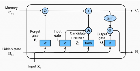
To put it briefly, the “LSTM” design consists of a set of memory blocks that are recurrently connected. The memory blocks maintain their state and oversee the control of information flow over time through the non-linear gating units. A typical “LSTM” block, as shown in Figure 6, includes gates, an input signal represented as x^(r), an output represented as y^(f), peephole connections, and activation functions. The output of the block forms recurrent connections with both the block input and all the gates.

image008.png

Figure 6. A typical vanilla “LSTM” block architecture

The working principle of the LSTM can better be understood by analyzing a network that comprises M inputs and N processing blocks. In this recurrent neural system, the forward pass can be explained thus:

Block Input: The major process of this step is updating the component of the block input which involves combining the current input, denoted as x^(r), and the output of the “LSTM” unit, y^(r-1), from the preceding iteration; this process can be expressed thus:

${{\text{z}}^{\left( \text{r} \right)}}=\text{g}\left( {{\text{W}}_{\text{z}}}{{\text{x}}^{\left( \text{r} \right)}}+{{\text{R}}_{\text{z}}}{{\text{y}}^{\left( \text{r}-1 \right)}}+{{\text{d}}_{\text{z}}} \right)$                                (35)

Input gate: The process here is the updating of the input gate that requires the incorporation of the output of the preceding “LSTM” unit y^(r-1), the current input x^(r), and the cell value c^(r-1) from the preceding iteration as represented in the following equation:

${{\text{i}}^{\left( \text{r} \right)}}=\text{ }\!\!\sigma\!\!\text{ }\left( {{\text{W}}_{\text{i}}}{{\text{x}}^{\left( \text{f} \right)}}+{{\text{R}}_{\text{i}}}{{\text{y}}^{\left( \text{r}-1 \right)}}+{{\text{p}}_{\text{i}}}\odot {{\text{c}}^{\left( \text{r}-1 \right)}}+{{\text{d}}_{\text{i}}} \right)$                           (36)

where, ⊙ is a point -wise multiplication of 2 vectors, W_i,R_i and p_i are the weights related to x^(r), y^(r-1) and c^(r-1), respectively, and d_i is the bias vector related with this specific component.

The “LSTM” layer is responsible for determining the data to be kept in the network's cell states from the previous step, represented as c^(r). This process requires the selection of the candidate values z^(f) to be added to the cell states, as well as the determination of the activation values z^(f) of the input gates.

Forget Gate: The major task in this phase is the determination of the data to be discarded from its prior cell states c^(r-1). This is achieved by computing the forget gate’s activation values f^(r) at time step t in consideration of the current input x^(r), the outputs y^(r-1), the memory cell’s state c^(t-1) from the previous time step (t-1), the bias terms b_f associated with the forget gates, and the peephole connections.

${{f}^{\left( r \right)}}=\sigma \left( {{W}_{f}}{{x}^{\left( r \right)}}+{{R}_{f}}{{y}^{\left( r-1 \right)}}+{{p}_{f}}\odot {{c}^{\left( r-1 \right)}}+{{b}_{f}} \right)$                            (37)

where, W_f, R_f and p_f are the weights of x^(r), y^(r-1) & c^(f-1), respectively; b_f is the bias weight vector.

Cell: During the cell stage, the calculation of the cell value entails incorporating the block input z^(r), input gate i^(r), and forget gate f^(r) values with the preceding cell value. This process can be expressed as follows:

${{\text{c}}^{\left( \text{r} \right)}}={{\text{z}}^{\left( \text{r} \right)}}\odot {{\text{i}}^{\left( \text{r} \right)}}+{{\text{c}}^{\left( \text{r}-1 \right)}}\odot {{\text{f}}^{\left( \text{r} \right)}}$                              (38)

Output Gate: Output Gate: The process here is to determine the output gate by merging the current input x^(r), the cell value c^(r-1) from the preceding iteration, and the output of the “LSTM” unit y^(r-1) as seen in the following relation:

${{\text{o}}^{\left( \text{r} \right)}}=\text{ }\!\!\sigma\!\!\text{ }\left( {{\text{W}}_{\text{o}}}{{\text{x}}^{\left( \text{r} \right)}}+{{\text{R}}_{\text{o}}}{{\text{y}}^{\left( \text{r}-1 \right)}}+{{\text{p}}_{\text{o}}}\odot {{\text{c}}^{\left( \text{r} \right)}}+{{\text{d}}_{\text{o}}} \right)$                          (39)

In the given equation, p_o, W_o and R_o are the weights of c^(r-1) x^(r) and y^(r-1), respectively, while b_o denotes the bias weight vector.

Block Output: In the end, the block output is computed by combining the current cell value c(t) with the current output gate value, as illustrated below:

$\text{y}\left( \text{r} \right)\text{ }\!\!~\!\!\text{ }=\text{ }\!\!~\!\!\text{ g}\left( \text{c}\left( \text{r} \right) \right)\text{ }\!\!~\!\!\text{ }\_\text{ }\!\!~\!\!\text{ o}\left( \text{r} \right)$                                    (40)

where, σ, g, and h are non-linear activation functions that are applied to each element.