Naga Jagadesh Bommagani*![]() | Manjunatha Basavannappa Challageri
| Manjunatha Basavannappa Challageri![]() | Nunsavatu V Naik
| Nunsavatu V Naik![]() | Hanumantha Rao Jalla
| Hanumantha Rao Jalla![]() | Syed Ziaur Rahman
| Syed Ziaur Rahman![]() | Anandhi Rajamani Jayadharmarajan
| Anandhi Rajamani Jayadharmarajan![]()
© 2024 The authors. This article is published by IIETA and is licensed under the CC BY 4.0 license (http://creativecommons.org/licenses/by/4.0/).
OPEN ACCESS
Breast tumors have become one of the most frequent illnesses among women, with 287,850 new cases projected to be discovered in 2022. Of those, 43,250 women passed away from this malignancy. The mortality rate for cancer might be decreased through early detection. Despite this, employing mammography photographs to manually identify this kind of cancer is a challenging process that always demands an expert. In the literature, a number of AI-based (Artificial Intelligence) strategies have been proposed. However, they still deal with issues including irrelevant feature extraction, inadequate training models, and similarities between cancerous and non-cancerous areas. In order to identify breast cancer, this research suggested an SMO-MAFNet-Hybrid Alexnet model. The images in this study were first preprocessed to get rid of noise. After that, the multi-attention fusion network (MAFNet) is used to extract features. The Spider Monkey Optimization (SMO) method is utilized in this work to optimize the learning rate in MAFNet. Following feature extraction, classification is done using the AlexNet model. In this work, hybrid optimization, namely Ant Colony Optimization-Reptile Search Algorithm (ACO-RSA), is applied to fine-tune the hyperparameters in AlexNet classification. The suggested method was tested using the CBIS-DDSM (Curated breast imaging subset of Digital Database for Screening Mammography) dataset and demonstrated an accuracy of 98%, outperforming previous models.
breast cancer, AlexNet, Spider Monkey Optimization, multi attention fusion network, hybrid optimization
Large connected gadgets link to the Internet of Things (IoT), an interactive paradigm that is constantly increasing and enabling communication between people and things in our current digital environment. IoT includes all medical devices that gather patient health information, including smartphones, smartwatches, wearable wristbands, integrated surgical instruments, and other flexible health monitoring gadgets [1]. This technology is used in both homes and hospitals to remotely monitor patients, facilitating the early diagnosis and treatment of serious illnesses and medical problems. Remote patient monitoring in hospital settings has the potential to drastically lower needless doctor visits, hospital stays, readmissions, and total healthcare expenses [2]. Despite the difficulties and barriers encountered in the past, IoT technologies have revolutionized the world of medical applications [3]. These IoT devices have the potential to provide large amounts of biomedical data, which may be very helpful in the creation of systems that automatically gather medical data [4]. As IoT devices are connected, big data, together with cutting-edge Machine Learning (ML) technology, plays a crucial role in improving current healthcare systems' diagnosis, treatment, and decision-making [5].
The Internet of Everything (IoE), which incorporates symptomatic treatments and monitoring along with tracking of patients, has attracted research attention as a result of IoT in biomedical applications [5]. The World Health Organization (WHO) ranks breast tumors as the most common worldwide reason for death in women. Early identification of breast tumors in women is the greatest approach to saving lives and reducing healthcare expenditures [6]. In general, cancers are classified as either benign or malignant. Benign tumors don't pose a life-threatening hazard, but they may make women more likely to develop breast cancer. On the other hand, malignant tumors are cancerous and need to be treated right away. According to research on breast cancer screening, 20% of women had malignant tumors [7]. Breast tumors may be identified over an extended duration of time by utilizing a number of methods, including X-rays, ultrasound, mammography, magnetic resonance imaging (MRI), positron emission tomography (PET), and computed tomography [8]. Breast cancer in its early stages may be assessed by screening, which finds the disease when small breast symptoms appear. Mammography, clinical breast exams, and other methods are additional methods for breast screening. In mammography, doctors utilize brief-intensity X-rays to scan the breasts for anomalies. There are two other imaging techniques to check for breast cancer issues: ultrasound and MRI scans [9]. A "one-size-fits-all" screening strategy runs the risk of underdiagnosing breast tumors, particularly in women with dense breasts. Breast density, which is the ratio of fibroglandular tissue to fatty tissue in the breast, affects the sensitivity of mammography [10]. Mammography has established as the most accurate approach for identifying breast tumors because of its capacity and affordability to meet medical needs. The major technique used by doctors to make diagnoses is mammography analysis, although this approach is subject to bias and physician fatigue [11].
The mammography technique has a poor rate in detecting breast tumors, which is unfortunate. Depending on the type of tumors, the general size of the female breasts, and the elder age of the victim, it may give false-negative results of 5% to 30% [12]. As a result, mammography uses low-dose radiography, which enables viewing of the internal breast tissue. Breast cancer is detected using a variety of signal processing techniques, such as curvelet transform, microwave imaging, and ultrasound imaging. The traditional approach for categorizing medical infections, such as skin blemishes, breast lumps, and brain tumors, is based on pattern recognition [13]. The mammography characteristics for breast cancer are manually retrieved, and they are then sent inside an ML classifier for categorization. Obtaining a proper classification, however, remains challenging because of many imaging difficulties and alterations in tumor regions. As a result, deep learning (DL) has played a major part in the past ten years in the detection and classification of medical infections, particularly for breast cancer [14].
Current techniques for identifying breast cancer from mammography pictures mostly depend on deep learning architectures or classic machine learning algorithms. Although these techniques have showed promise, they frequently fail to capture the complex patterns and nuanced characteristics typical of breast cancer in its early stages. Additionally, they can be less effective in clinical situations due to noise and fluctuations in image quality.
By utilizing cutting-edge approaches in deep learning and attention mechanisms, the suggested method, "Detection of Breast Cancer in Mammogram Images using Multi-Attention Feature Extraction with Hybrid RSA-based AlexNet," seeks to overcome these drawbacks. The major contributions in this paper are:
Organization of the work
Section 2 reviews the relevant works, Section 3 offers a brief description of the proposed model, Section 4 illustrates the results and testing analysis, and then Section 5 delivers the results in pictorial form and tabulation with conclusion.
In their study, Pati et al. [15] created a deep transfer learning (DTL) model-based autonomous system for identifying breast cancer. For their investigation, they used mammography pictures from the publicly available online archive the cancer imaging archive (TCIA). Preprocessing was done on the data before it was entered into the model. In order to improve predictive accuracy (ACC), the study combined well-known deep learning (DL) techniques, such as support vector machine (SVM) classifiers and convolutional neural networks (CNNs), with transfer learning (TL) methods, specifically by utilizing models like Inception V3, ResNet50, VGG16, AlexNet, and VGG19. The research extensively used simulations to test the viability of their suggested strategy, evaluating several performance metrics and network indicators. Notably, the large collection of mammography pictures was divided into benign and malignant categories. With percentages of 97.99%, 99.51%, 98.43%, 80.08%, and 98.97%, respectively, for precision (PR), sensitivity, specificity, F1 score, and accuracy, the findings outperformed earlier mammography-based studies. The report also described the use of fog computing technology, which improves system performance while reducing the load on core servers and upholds strict criteria for patient privacy and data security.
Specifically, for IoT applications, Rajeswari et al. [16] set out to construct an exponential honey badger optimization-based deep convolutional neural network (EHBO-based DCNN) with a major emphasis on early breast cancer (BC) diagnosis. They cleverly combined the Honey badger optimisation (HBO) strategy with the exponential weighted moving average (EWMA) method to produce the EHBO approach, which they used to achieve their goal. The EHBO framework was painstakingly created to enable the smooth transfer of medical data collected through IoT to a central base station (BS) and at the same time identify important cluster heads to discover instances of BC. The study then used data augmentation methods, texture analysis, and the extraction of statistical features. The implementation of a deep convolutional neural network (DCNN) for BC classification was the last phase. With test scores of 0.9029, 0.9051, and 0.8971, respectively, the algorithm demonstrated remarkable performance, attaining impressive levels of specificity, sensitivity, and total accuracy. The multi-layer perceptron (MLP), deep learning (DL), support vector machine (SVM), and ensemble-based classifier were all outperformed by this suggested approach, with margins of 7.23%, 6.62%, 5.39%, and 3.45%, respectively.
Kwak et al. [17] used DL methods for medical image identification in their study to dive into the field of breast cancer detection. Their in-depth investigation included a variety of medical imaging modalities, including histology, ultrasonography, and X-ray (Mammography) pictures. This thorough investigation's main goals were to improve breast cancer detection precision and give accurate identification of afflicted anatomical areas. The main objective was to improve the detecting process's overall accuracy. A wide range of image classification techniques were investigated by the researchers, including VGGNet19, ResNet50, DenseNet121, and EfficientNet v2. They also explored the world of picture segmentation technologies, analyzing choices including UNet, ResUNet++, and DeepLab v3. Furthermore, the research dug into the evaluation of numerous loss functions, including binary cross-entropy, dice loss, and Tversky loss, as ways to improve the analysis. A variety of data augmentation methods were carefully used to expand the dataset and strengthen the validity of their conclusions.
Park et al. [18] designed to evaluate the capability of an ML system in predicting axillary lymph node (ALN) metastasis by incorporating preoperative contrast-enhanced computed tomography (CECT) data from both the main tumour and ALN. The study included 266 breast cancer patients who received pretreatment CECT scans of their chest cavities at a single medical facility. The study included a variety of ML methods, such as extreme gradient boosting (XGBoost), random forests, and neural networks (NN). The researchers included statistical analysis with recursive feature elimination (RFE) as part of the ML process. With an ACC of 0.74 and an Area Under the Receiver Operating Characteristic Curve (AUROC) of 0.12, the NN with RFE model was shown to be the most successful ML model for predicting ALN metastases in breast cancer. The contrast between a model without these properties and a NN with RFE model adding ALN characteristics from CECT was particularly remarkable. The former consistently outperformed the latter across all evaluation criteria, highlighting the significant benefit of integrating ALN features in the model. By using contrast-enhanced computed tomography (CECT) images from both the original tumour and axillary lymph nodes, this research illustrates how well ML methods predict ALN metastasis. These results demonstrate ML's outstanding capability to distinguish between benign and malignant ALNs, offering helpful information for therapeutic decision-making in the treatment of breast cancer.
An IoT-based automated method for diagnosing breast cancer was created by Gao and Rezaeipanah [19]. When a suspect patient is examined using IoT-enabled medical equipment, this cutting-edge device quickly communicates medical pictures to a data warehouse. The ability to precisely analyze these medical pictures by radiologists was enabled by the researchers' use of four pre-trained CNN models, notably InceptionResNetV2, InceptionV3, VGG 19, and ResNet 152. To combine these models for greater accuracy, they used an ensemble classifier. Additionally, algorithms were used to offer accurate predictions in three separate categories: pneumonia patients, healthy people, and women with breast tumors. The research used two separate datasets, each of which had CT-scan and X-RAY pictures. Notably, the InceptionResNetV2 architecture attained a remarkable accuracy rate of 99.36% for CT-scan pictures whereas the Inception V3 model showed an exceptional accuracy rate of 96.94% for X-RAY images. These discoveries have the potential to improve patient care by enabling healthcare workers to identify breast tumors early on and so minimizing the need for frequent doctor visits, which would lessen the burden on healthcare facilities.
The combination of several CNNs and meta-learning algorithms was researched by Ali et al. [20] to create a trustworthy and efficient breast cancer classification model. A sizable database of breast ultrasound images (BUSI), which included a range of breast abnormalities, was used in the investigation. The major objective was to identify these tumors' malignant or benign status, an essential step in the early detection and quick treatment of breast cancer. The complicated and varied composition of the images presented a challenge to current ML and DL techniques. To completely resolve this issue, the research team proposed a novel model integrating cutting-edge techniques such as meta-learning ensemble approach, transfer learning, and data augmentation. The model's use of meta-learning to accelerate learning and provide speedy adaptation to new datasets was its primary strength. Utilizing pre-trained models like Inception, ResNet50, and DenseNet 121 further helped the model's capacity to extract features. The dataset was augmented with artificially created training images to increase its size and diversity. Notably, the model improved classification accuracy (ACC) by combining the outcomes of several CNNs utilizing meta ensemble learning techniques. As part of the research methodology, the BUSI dataset was preprocessed, and different CNNs with various architectures and trained models were trained and assessed. After employing a meta-learning technique to refine the learning process, ensemble learning was used to merge many CNN outputs. The study's results provided significant new information about the proposed model in addition to confirming its correctness and effectiveness. The research team conducted a thorough investigation, compared their model's F1 score, ACC, recall (RC), and precision-recall (PR) measurements with cutting-edge methods employed in current systems.
Thirumalaisamy et al. [21] developed a novel approach to aid radiologists in detecting breast cancer more rapidly. This approach includes synthesized convolutional neural networks (CNNs), an enhanced optimization strategy, and transfer learning. A crucial part of this technique was modifying the ant colony optimization (ACO) method to fit the limitations of opposition-based learning (OBL). The researchers used the enhanced ant colony optimization (EACO) technique to tune the hyperparameters of the CNN architecture. The EACO-ResNet101 model was developed inside this unique framework by combining the ResNet101 CNN architecture with the EACO algorithm. Experiments were conducted using mammographic datasets from MIAS and DDSM (CBIS-DDSM) to evaluate the efficacy of this method. The suggested model performed better, according to the CBIS-DDSM dataset findings, which had ACC rates of 98.63%, sensitivity rates of 98.76%, and specificity rates of 98.89%. The model performed quite well on the MIAS dataset as well, with a classification ACC of 99.15%, a sensitivity of 97.86%, and a specificity of 98.88%. These findings unequivocally show that, as compared to older techniques, the EACO-ResNet101 model performs better in breast cancer diagnosis.
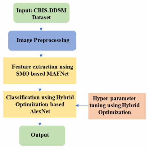
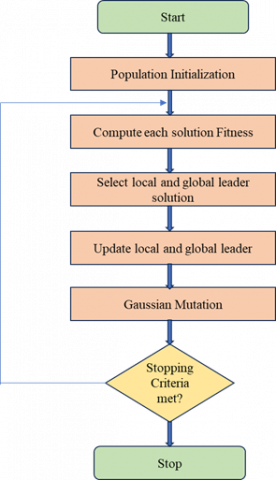
Figure 1 depicts the stages involved in putting the proposed approach into action. The section (workflow) contains image preprocessing, feature extraction using SMO based MAFNet and hybrid optimization based AlexNet feature classification.
Figure 1. Workflow
3.1 Dataset description
The study conducts an in-depth analysis utilizing data extracted from 1459 mammograms sourced from the Curated Breast Imaging Subset of the Digital Database for Screening Mammography (CBIS-DDSM). The CBIS-DDSM dataset represents an enhanced version of the Digital Database for Screening Mammography (DDSM), which is widely recognized and utilized in breast cancer research and diagnostics. This upgraded manifestation, the CBIS-DDSM dataset, comprises a diverse range of mammographic images annotated with detailed information regarding various abnormalities and lesions.
Within the CBIS-DDSM database, a comprehensive array of mammogram images is categorized based on the presence and nature of abnormalities. Specifically, the dataset encompasses 398 images depicting benign calcifications, 417 images illustrating benign masses, 300 images showcasing malignant calcifications, and the remaining images displaying malignant masses. These classifications provide a nuanced representation of different pathological conditions and abnormalities commonly encountered in mammography screenings.
All images contained within the CBIS-DDSM dataset adhere to a standardized format, with dimensions set at 224 × 224 pixels and encoded in the RGB (Red, Green, Blue) color space. This uniformity ensures consistency in image resolution and format across the entire dataset, facilitating streamlined data preprocessing and analysis procedures. Table 1 in the study provides a comprehensive overview of the dataset, summarizing key characteristics and distribution statistics pertaining to the different categories of abnormalities represented within the CBIS-DDSM database. This summary serves as a valuable reference for researchers and practitioners involved in the field of breast cancer detection and diagnosis, offering insights into the composition and diversity of the dataset under scrutiny.
Overall, the utilization of the CBIS-DDSM dataset in the study underscores the importance of leveraging high-quality, annotated data repositories to drive advancements in medical imaging research, particularly in the context of breast cancer detection and diagnosis. The dataset's richness in pathological variations and standardized image attributes empowers researchers to develop and validate robust algorithms and methodologies aimed at improving the accuracy and efficiency of breast cancer screening and prognosis.
Table 1. Dataset description
|
Name |
Description |
|
Total Number of Images |
1459 |
|
Color Grading |
RGB |
|
Benign Classification |
398 |
|
Benign Mass |
417 |
|
Malignant Mass |
344 |
|
Malignant Classification |
300 |
|
Dimension |
224×224 |
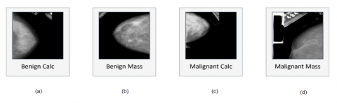
After receiving the dataset, several photos that were just artifacts labeled as malignant masses or blank images were discovered. ACC might suffer as a result of these photographs. 17 photos were therefore manually eliminated. 327 malignant mass mammograms remained in the photos after the photographs had been removed, whereas the number of mammogram images in the other categories remained steady. As a consequence, 1442 photos in a dataset with four distinct classifications are produced. Examples of four classes are shown in Figure 2, along with information on their traits and artifacts.
Figure 2. Dataset (CBIS-DDSM) comprising mammograms having four classifications in which multiple artefacts appear in each class
Figures 2(a) and (b) both include a little label at the bottom edge of the picture, a huge label in Figure 2(b), a pair of straight lines linked towards the image's breast region in Figure 2(c), and a straight line at the bottom edge of Figure 2(d).
3.2 Preprocessing
Before inserting the pictures inside a neural network for analysis, image pre-processing thought to be the most crucial operation to attain a reasonable level of ACC and shorten the computing time of a model. It is complicated to an artificial neural network technique in order to categorize mammograms without first using pre-processing methods. As a result, picture pre-processing is done first. The studies [22, 23] outlined many pre-processing methods that may be used without degrading the quality of the original picture. Two further research [24] improved the contrast of mammography using tried-and-true techniques.
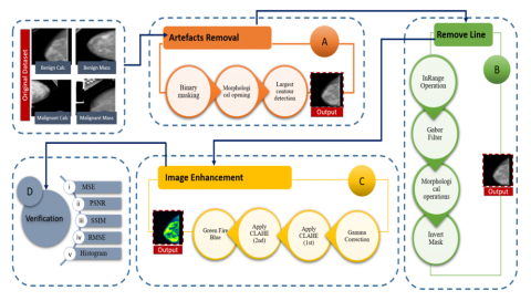
In this part, it is explained how mammography quality and quantity might be improved. This covers picture improvement, background removal, and artifact removal. The primary processes, related sub-processes of picture pre-processing phase are shown in Figure 3. Artefact removal, remove line, picture enhancement, and testing are the primary procedures.
Figure 3. Phase chart of image pre-processing where every process is depicted with a structure of blocks
Block (A): A variety of approaches are used to remove any anomalies seen in original mammograms as: binary masking of the image, morphological opening (second process), and largest contour identification that produce artefact at ease mammograms; In block (B) lines are connected with the female breast portion of the mammograms eliminated via different techniques: in Range Operation(the early process) following Gabor filter, Morphological opening, which is the third process and then Invert mask manipulation; (C) image enhancement through further Gamma correction following, 1st then 2nd contrast limited adaptive histogram equalization and Green Fire Software with a Blue Filter, which is ImageJ; subsequently in the block (D) the ACC of modified pictures has been examined by image statistical evaluation.
To get a more accurate result, artifacts from the mammograms are first eliminated, then certain techniques (binary masking of images, followed by process of morphological opening process, and biggest contour identification, the final phase) are used. Second, the vertical line connected to the breast region is removed using the "remove line" step. In this study, techniques including Range operation, Gabor filter morphological operation subsequently inverse masking methods were applied. The subprocesses of opening and dilatation are both part of the morphological operation. Thirdly, image enhancement is used to boost the contrast and luminosity of the initial pictures in order to improve the visibility of the malignant condition. Gamma correction, which is depicted in the block image [25], CLAHE (1st process) [26], CLAHE (2nd process), and the green-coloured fire blue ImageJ filtering [27] are the subprocesses of this stage2. An increase in visibility may be seen after using CLAHE. Then, CLAHE is used once again to boost the contrast. In other words, the method involves applying CLAHE twice. CLAHE should not be used a third time since doing so might distort the contrast level and impair the ability to see fine details in mammograms. Finally, in the verification step, evaluation methods are performed to the processed pictures to analyze the outcomes, including PSNR (peak signal-to-noise ratio), MSE (mean square error), RMSE (root mean squared error), SSIM (structural similarity index) and histogram analysis. Figure 3 depicts the entire pre-processing pipeline, with the result of each stage serving as the input for the next stage.
3.3 Feature extraction using SMO based MAFNet
3.3.1 MAFNet architecture
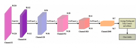
As a feature extractor, multi-attention fusion CNN (MAFNet) technique is used in this research. Four convolution models are present in the centre of MAFNet's $1 \times 1 \times 1$ convolution layers [28], while three convolution frameworks are found throughout all the modules. And the distribution of the convolution module follows a symmetrical pattern similar to [29]. Finally, there are 26 convolution modules in the FC layer [30, 31]. Following that, the pictures are supplied as input, and the first $1 \times 1$ convolutional method is carried out. 4 convolution algorithms are subsequently passed for four times again. The contextual transformer (CoT) block of the primary ResNet (Residual Network) convolution structures replaces $3 \times 3$ convolutional operation. The characteristics recovered are next provided as feed to FC levels (layers), which carry out the function of "classification" in neural network approach, following the early convolution, pooling, and excitation procedures [32]. Figure 4 depicts the MAFNet model's architecture. To assess the likelihood of categorization, it also uses the Softmax function. The outcome resulting from the classifier's results is finally provided as below.
$Softmax\left(z_j\right)=\frac{e^{z_i}}{\sum_{i=1}^n e^{z_i}}$ (1)
Figure 4. Architecture of MAFNet
Eq. (1) exhibits the total number of groups or classes, $z_j$ indicates result value for jth node, $z_i$ denotes the result value of ith node, while e indicates the fundamental constant, which may be computed as follows.
$S L_{C E}=-\sum_{i=1}^N l_i \log p_i$ (2)
The variable li in Eq. (2) refers to the thermal encoding of individual tags i from the set $\mathrm{i}(0, \ldots, \mathrm{N}-1)$. When li equals 1, it implies that the ith tag is present among the labels, while all other labels are set to zero. N also reflects the total number of tags present. The prediction probability associated with the ith label is represented by pi which corresponds to the Softmax score when the target label is i.
This needs to be observed that a lower learning rate could conclude in less rapid integration, while the maximum learning rate might end up resulting in a continuous fluctuation of loss function. When trying to construct a system with outstanding ACC and optimal variables accompanied with quick learning, an adjustable learning rate technique is used, which allows the learning rate to be adjusted every thirty epochs, where calculation appears below [33].
$l r=l r_0 \times 0.1^{\frac{epoch}{30}}$ (3)
In Eq. (3), lr signifies the current learning rate, lr0 indicates the main learning rate, while epoch denotes the whole number of training cycles.
3.3.2 Learning rate optimization using SMO
Spider Monkey Optimization (SMO) plays an essential role in optimizing the learning rate (lr), as specified in Eq. (3). The SMO technique is a metaheuristic approach that was inspired by the social behavior of spider monkeys. This novel approach to problem solving draws on the collective behaviors of spider monkeys, integrating features of fission and swarm intelligence, as mentioned in the studies [34, 35]. Spider monkeys reside in communities between 40 and 50. A leader divides the responsibility of finding food in a community. Typically, a spider monkey swarm consists of 40 to 50 individuals, and the leader divides out the responsibility of finding food within an area. The worldwide leader of the swarm in the case of a food scarcity is always a leading female, which results in changeable smaller groupings. Based on the food supply in a particular area, the group size is determined. The spider monkey's size is closely correlated with the amount of food available. The required requirements are satisfied by the SMO-based approach of swarm intelligence (SI).
Smaller groups are formed to share the spider monkeys' foraging tasks. Self-organization: The group size is used to determine the food availability requirement. Intelligent foraging activity results in an intelligent choice. Swarm is used to start the food hunt. The distance between persons serving as food sources is computed. The distances between the members of the food groups change the locations for choosing. It is calculated how far apart individual is from their food supply.
Figure 5. Flowchart of SMO
For its six iterative collaborative stages, the SMO approach relies on trial and error: global leader decision phase, learning phase, local leader learning phase, local leader decision phase, global leader and local leader phase. ACO algorithms, inspired by the foraging behavior of ants, excel in exploring complex search spaces and identifying optimal solutions through iterative interactions. The collaborative framework of hybrid ACO-RSA enhances the robustness and generalizability of AlexNet by mitigating the risk of model bias and overfitting. By leveraging diverse optimization strategies, the model can effectively adapt to variations in mammogram images and generalize its diagnostic capabilities across diverse patient populations and imaging conditions.
In summary, the selection of SMO for MAFNet and the integration of a hybrid ACO-RSA approach with AlexNet reflect a strategic fusion of bio-inspired optimization techniques tailored to the unique requirements of breast cancer detection in mammogram images. These algorithmic choices contribute to the development of robust, efficient, and clinically relevant detection frameworks, ultimately advancing the field of medical image analysis and improving patient outcomes in breast cancer diagnosis and treatment. This approach's workflow is shown in Figure 5.
Below is a detailed explanation of the SMO approach.
Initializing
Population $P$ of spider monkeys are distributed using the SMO technique, where $S M_p$ stands for the $p-t h$ monkey in the population and $p=1,2 \ldots P$. The entire number of variables in a monkey is $M$, making them an M-dimensional vector. Using Eq (4), one potential response to each $S M_p$.
$S M_{p q}=S M_{minq }+U R(0,1) \times\left(S M_{maxq }-S M_{minq }\right)$ (4)
where, $S M_{p q}$ is $p t h S M$ of $q t h$ dimension. $S M_{p q}$ lower and upper bounds are $S M_{\text {ming }}$ and $S M_{\text {maxg }}$ in the $q t h$ direction for random number of $U R(0,1)$ uniform distribution is within the range of $[0,1]$.
Local Leader Phase (LLP)
LLP is an important part of the process in which SM, the local leader, changes the current location based on previous occurrences involving local group members. This change is done to improve the applicability of the new site in comparison to the prior one. The decision to relocate SM is conditional on the new site's fitness value exceeding that of the existing location. Eq. (5) provides the formula for updating the location of the $p t h$ SM within the lth local group.
$\begin{gathered} SMnew_{p q}=S M_{p q}+U R(0,1) \times\left(L L_{l q}-S M_{p q}\right)+ U R(-1,1) \times\left(S M_{r q}-S M_{p q}\right)\end{gathered}$ (5)
The symbol for the $q$ th dimension's $l$ th local group leader location is $L L_{l q}$.The qth dimension's $l$ th local group of the lth $S M$ is chosen at random and is designated as $S M_{r q}$, where $r, p$.
Global Leader Phase (GLP)
The local group members' input and the global leader's insights are used to guide the location improvement process, which is carried out in accordance with the LLP. Eq. (6) is used to calculate the new location data.
$\begin{gathered}SMnew_{p q}=S M_{p q}+U R(0,1) \times\left(G L_{l q}-S M_{p q}\right)+U R(-1,1) \times\left(S M_{r q}-S M_{p q}\right)\end{gathered}$ (6)
where, $q$ th dimension of global leader location is denoted as $G L_{l q}$ and an arbitrarily selected index is $q=1,2,3, \ldots M$.
In this step, the SM fitness determines probability prbp. Based on the probability value, the location of $S M_p$ is updated, and a better site’s candidate can allow to a variety of opportunities to enhance convergence. Eq. (7) provides the probability calculation results.
$p r b_q=\frac{f n_p}{\sum_{p=1}^N f n_p}$ (7)
where, $p t h$ $S M$, the symbol for fitness value is $f n_p$. A comparison is made between the SMs' new location fitness and their prior location. The location's top fitness value is taken into account.
Global Leader Learning (GLL) Phase
The global leader location has been updated by using a greedy approach. New spider monkey’s position is based upon world leader position for optimum population viability. The ideal site is used to apply the global leader. There is a 1 increment added to Global Limit Count in the event of updates.
Local Leader Learning (LLL) Phase
The local group and a greedy selection method are used to update the position of the local leader. The SM location is modified to guarantee the local leader's ideal placement inside a particular local group. The local leader's position is then precisely adjusted to ensure success. The local limit count is raised by one if no new entries are found.
Local Leader Decision (LLD) Phase
Local group candidates alter location at random in accordance with step 1 if the local leader can’t able to alter the position or uses the existing data from the global and local leaders based on the Eq. (8).
$\begin{array}{r}SMnew _{p q}=S M_{p q}+U R(0,1) \times\left(G L_{l q}-S M_{p q}\right) +U R(0,1) \times\left(S M_{r q}-L L_{p q}\right)\end{array}$ (8)
Global Leader Decision (GLD) Phase
If the position is not changed for a global leader up to the GLL, according to the preferences of the global leader, the populace is split into smaller sections. After receiving a maximum number of groups (MG), the splitting procedure begins. Each time, a local authority figure is chosen for recently established group. The greatest number of permissible sets is formed, and the global leader remains in their position until the pre-fixed permitted limit has been attained. At that point, the global leader seeks to combine all permitted groups into an individual group. The largest number of permissible chains is formed, and the global leader holds on to that position until the pre-fixed maximum has been reached. At that point, the global leader seeks to combine all permitted chains to unite. The following are the SMO evaluating control specifications:
Rate of perturbation (pr);
Maximum number of groups (MG);
Global Leader Limit;
Rate of Local Leader Limit.
Gaussian Mutation
In difficult iterative optimization situations, the SMO approach gets stymied in a local optimum. The algorithm solution value does not vary throughout iteration. This strategy leaves the location of the local optimum and includes stochastic perturbation and the Gaussian mutation before continuing on executing the creed in order to enhance the algorithm probability and algorithm deficiency. Eq. (9) displays the Gaussian mutation.
$x^{i, i t e r+1}=\left\{\begin{array}{cc}x^{i, i t e r}+rand & \text { if } r \geq 0.2 \\ x^{i, iter } \times Gaussian(\mu, \sigma) & \text { otherwise }\end{array}\right\}$ (9)
where, $r j$ is random fluctuation and $r a n d$, a randomized number between the interval of $[0,1]$. The dispersion of Gaussian variance is given in Eq (10).
$Gaussian(\mu, \sigma)=\left(\frac{1}{\sqrt{2 \pi \sigma}}\right) \exp -\left(\frac{(x-\mu)^2}{2 \sigma^2}\right)$ (10)
where, $\sigma^2$ and $\mu$ are denoted for variance and mean value.
3.4 Classification using hybrid optimization based AlexNet
3.4.1 AlexNet model
When features that had been extracted, the AlexNet CNN DL architecture has been used in the proposed study to classify breast cancer. The network's architecture has 5 convolution layers, which are followed by an average of 3 pooling layers, making it deeper than ordinary CNN. To prevent data overfitting, a dropout percentage of 0.5% has been assigned to the entirely linked layers present. The following elements make up the architecture:
• 1 Convolution with 11 × 11 kernel size (1CONV)
• Rectified Linear Unit Layer Activation (RELU)
• 3 Maximum Pooling (3 × 3)
• 1 Maximum Pooling (4 × 4 kernel)
• Rectified Linear Unit Layer Activation (RELU)
• Rectified Linear Unit Layer (RELU)
• Response Normalization Layer
• Rectified Linear Unit Layer (RELU)
• Rectified Linear Unit Layer Activation (RELU)
• 4 Convolution with 3 × 3 kernel size
• Rectified Linear Unit Layer Activation (RELU)
• 2 Convolution with 5 × 5 kernel size (2CONV)
• Fully Connected Layer (4096 nodes)
• 2 Maximum Pooling (3 × 3)
• Fully Connected Layer (4096 nodes)
• 3 Convolution with 3 × 3 kernel size (3CONV)
• Soft-max out
Figure 6. AlexNet CNN architectural layout of the proposed technique
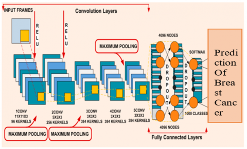
This research is built on the suggested AlexNet CNN framework, which is shown in Figure 6. The first picture input layer serves as a preprocessing step for the study project. The spatial dimensions of incoming frames are down-sampled from 640 × 480 to 227 × 227, thereby lowering the processing requirements of the DL architecture. The architecture is made up of five convolutional (CONV) layers, three pooling (POOL) layers, and a rectified linear unit (RELU) after each. A total of 96 kernels with size of 11 × 11 by 3 are used in the first convolutional layer. The second convolutional layer then makes use of 256 kernels that are 5 × 5 in size. 384 kernels with 3 × 3 dimensions are selected for the third, fourth, and fifth layers. An activation map is produced for each convolutional layer. A 2 × 2 stride is used to merge the activation maps (feature maps) from the first, second, and fifth convolutional layers with the 3 × 3 pooling layers. The framework is divided into eight levels, each containing 4096 nodes. These layers are essential for building flexible feature maps that make feature extraction easier. Then, the fully connected layers (FC) get the activation maps, and Soft-max activation is used to generate classification probabilities, which are then used in the final classification step.
Convolution Network Layer
The layer that creates the activation maps that is exposed to classification layers in the DL phenomenon of neural networks is the most important layer. It contains kernel which moves across the source frame (input) to produce the activation map as the output. Everywhere the input, matrix multiplication was done, and the result was then integrated. Eq. (11)'s output activation map is described as:
$N_x^r=\frac{N_x^{r-1}-L_x^r}{S_x^r}+1 ; N_y^r=\frac{N_y^{r-1}-L_y^r}{S_y^r}+1$ (11)
where, $\left(N_x, N_y\right)$ is the width along with the height of activation map that is output for the final layer, $\left(L_x, L_y\right)$, size of kernel and $\left(S_x, S_y\right)$ which determines the amount of pixels omitted by kernel in both vertical and horizontal lines and $r$, index denotes the level or layer i.e., $r=1$. Convolution is performed on the activation map being input and a kernel to produce resultant activation map that is described as:
$X_1(m, n)=(J * R)(m, n)$ (12)
where, $X_1(m, n)$ is a $2 \mathrm{D}$ output activation map created on combining the 2D kernel $R$ of magnitude $\left(L_x, L_y\right)$ and input activation map $J$ as indicated in Eq. (12). The symbol * denotes the convolution around $J$ and $R$. In Eq. (13), the convolution process is defined below;
$X_1(m, n)=\sum_{p=-\frac{L_x}{2}}^{p=+\frac{L_x}{2}} \sum_{q=\frac{L_y}{2}}^{q=+\frac{L_x}{2}} J(m-p, n-q) R(p, q)$ (13)
In the proposed structure, the utilization of 5 CONV layers along with RELU layer and response normalization layer for obtaining the highest activation maps generate the input frames needed to train the dataset with optimum ACC.
Rectified Linear Unit Layer
RELU activation technique is applied to each of the versatile layers in the next step in order to make the network non-linear and reinforce it. It effectively compensates regarding non-linear characteristics. It is employed to the map of features produced by the convolutional layer as the output. feature map. With regard to training time, the nonlinear slope descent becomes saturated by the usage of tanh(.) and the RELU activation function. Eq. (14) describes tanh(.) as:
$\begin{gathered}X_2(m, n)=\tanh \left(X_1(m, n)\right)=\frac{\sinh \left(X_1(m, n)\right)}{\cosh \left(X_1(m, n)\right)}=1+ \frac{1-e^{-2 * X_1(m, n)}}{1-e^{-2 * X_1(m, n)}}\end{gathered}$ (14)
where, $X_2(m, n)$ is a $2 \mathrm{D}$ result activation map by performing $\tanh ($.$) to the source activation map X_1(m, n)$ that is acquired after sent via the convolutional layer. The parameters used in the last activation map are acquired using RELU procedure as mentioned below:
$X(m, n)=\left\{\begin{array}{cc}0, & \text { if } X_2(m, n<0) \\ X_2(m, n), & \text { if } X_2(m, n \geq 0\end{array}\right\}$ (15)
where, $X(m, n)$ is derived by adapting the negative numbers to zero and gives the identical number again on obtaining any affirmative result which is demonstrated in Eq. (15). Inclusion this RELU layer into the design that was proposed as deep CNNs obtain substantially faster pace when integrating this specific layer (RELU).
Maximum Pooling Layer
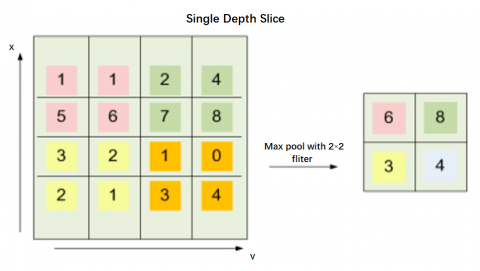
In order to decrease the relative dimension of every frame and the computational cost of the recommended DL structure, a layer is that is added to the suggested framework (pooling layer) despite the primary and next convolution layers and then again following the fifth convolution layer. The pooling method typically averages each slice of the picture or simply selects the highest value. The suggested method employs pooling, which produces superior results on this configuration, by utilizing the maximum value against each slice. Figure 7 shows how to activate the output for down-sampling the pictures while using the maximum pooling layer.
Figure 7. Maximum pooling layer
Response Normalization Layer and the SoftMax Activation
After the first two sessions, response normalization is carried out to decrease the rate of error on a test set of the recommended system. Along with the data input of the whole network in Eq. (16), this particular layer normalizes the layers of input inside systems. The process of normalizing works as described below:
$N_{e, q}^x=\frac{b_{e, f}^x}{\left(z+\alpha \sum_{j=\max (0, x-c / 2)}^{\min (T-1, x+c / 2)}\left(b_{e, f}^x\right)^2\right)^\gamma}$ (16)
where, $N_x, e, f$ indicates the normalization of the behavior of neurons $b_{e, f}^x$ that is estimated at location $(e, f)$ using the help of the kernel, k. $T$ is the entire spectrum of kernels inside the different layers. $z, c, a, g$ are the consistent values hyperparameters and the values they hold are modified through applying a set of validation parameters correspondingly.
A classifier on the top of the retrieved characteristics is called Soft-max. For classification of multiclass, the output of deep convolutional network layer (DCNN) is supplied to layer Softmax, which aids in calculating classification probabilities, after five sets of convolutional network layer processing. The last classification layer utilizes these probabilities in order to divide each frame into crowd/out-field, close-up, medium and long perspectives.
Dropout Layer
To avoid excessive fitting of the input information by raising the number of iterations by a ratio of two, keeping the neurons densely packed the dropout layer is implemented in the initial pair of layers that are completely connected once the number of iterations twice in the network. It employs neural networks to average models, and it is a particularly effective technique of managing training data. The generated activation map is down sampled to a single frame (pixel) for every map by the processing of maximum pooling layers, convolutional layer kernel sizes, and their skipping factors. The output of the uppermost layers is further related to a 1D feature vector through a layer that is completely connected. In order to extract higher-level characteristics from the training data, the top layer must always be properly connected to the output unit for the class label. This method, a normalization approach on completely linked layers prior to and subsequent dropout is illustrated.
3.4.2 Hyper parameter tuning using hybrid optimization
Ant colony optimization
Ant colony optimization (ACO) is an organically designed MA which imitates the ant's foraging behavior. Since ACO permits parallel processing without creating a process dependence and provides feedback on ant behavior in the search space, the model is more rational than previous MAs [36]. Ants can determine the quickest path between their colony and a food source; therefore, they are not blind while searching for food. Ants drop down a chemical substance known as pheromones along their trails as they go. The pheromone acts as a conduit to facilitate interaction amongst ants and indicates the shortest approach to their food source of food. Ants find food on detecting the pheromones left behind by other ants who have already travelled a certain route, which enhances the likelihood that more ants will follow in their footsteps. ACO bases its probabilistic judgments on the heuristic data and pheromone trail. As they go along a trail, the ants adjust the pheromone amount at any point. A feature has a greater chance of becoming a component of the shortest route the more ants pass over it and the more pheromones are deposited there as a consequence. The most ants will go down the route with the greatest concentration of pheromones, and it will also be the shortest way. Ants have distributed arbitrarily among a group of features corresponding to a predetermined greatest number of several generations $T$ and the pheromone level $t 0=1$ is initiated in each of the features of $M$. The change in probability $T P_i^k(g)$ of the $k t h$ ant at the ith feature in Eq. (17) has shown below [37].
$T P_i^k(g)=\left\{\begin{array}{lr}\frac{\left[\tau_i(g)\right]^\alpha\left[\eta_i\right]^\beta}{\sum_{j \in_{j i}^k}\left[\tau_i(g)\right]^\alpha\left[\eta_i\right]^\beta} & \text { if } j \in j_i^k \\ 0, & \text { otherwise }\end{array}\right\}$ (17)
where, $j_i^k$ is a collection of probable neighbors of $i$ th features that aren't examined using the $k t h$ ant. The relative relevance of pheromone intensity $t i$ and heuristic information $h j$ with regard to ants' actions are given by non-negative constants $a$ and $b$, correspondingly. On selecting an additional feature in the ant's route, a function of fitness (FF) is applied to measure the fresh set of chosen features. The progression of $k t h$ ant is terminated if the increase in the fitness value is not obtained after inserting any additional feature. In Eq. (18), if the halting requirement is not fulfilled, the quantity of pheromone level at succeeding generation $g+1$ at $i t h$ feature is upgraded as
$\tau_i(g+1)=(1-p) \tau_i(g)+\sum_{k=1}^N \Delta \tau_i^k(g)$ (18)
$\Delta \tau_i^k(g)=\left\{\begin{array}{lc}\left.F F\left(S_{k(g)}\right) / \mid S^k(g)\right) \mid, & \text { if } i \in S^k(g) \\ 0, & \text { otherwise }\end{array}\right\}$ (19)
where, $\mathrm{p}$ serves as the pheromone decaying rates, $0 \leq p \leq 1$ N represents the count of ants, $S^k(g)$ represents number of the chosen features, then Dtik stands for the pheromone dropped by $k t h$ ant if $i t h$ feature is along the simplest route of ants; if not it equals 0; which is mentioned in Eq. (19).
The stoppage criteria are accomplished whenever $g$ hits the preset threshold $T$. The set of features having the greatest pheromone level and least fitness score will be chosen as an OFS.
Reptile search algorithm
To mimic the surrounding and hunting behavior of crocodiles, [25] suggested the reptile search algorithm (RSA) in 2021. It represents a gradient-free technique that may commences with producing the following random responses to Eq. (20):
$x_{i, j}=rand_{\in[0, N]} \times\left(U B_j-L B_j\right)+L B_j$ for $i \in\{1, \ldots, N\}$ and $j \in\{1, \ldots, M\}$ (20)
where, $x_{i, j}$ is its $i$ th response for $j$ th source feature for entire $N$ responses containing $M$ features, $\operatorname{rand}_{\epsilon[0, N]}$ is an arbitrary integer dispersed similarly in the interval $[0,1](0,1)$, then this $j t h$ feature comprises upper $U B_j$ and lower $L B_j$ limits.
RSA may be defined in terms of two principles: exploration and exploitation, much as the other nature-inspired MAs. The crocodile's ability to makeover while surrounding its prey helps to explain these concepts. To benefit from crocodiles' natural behavior, RSA's total iterations are split into four phases. RSA completes the investigation in the first two phases using an encircling habit that includes high and belly walking motions. Crocodiles start to circle the area to explore it, enabling a more thorough search of the solution space. Eq. (21) may be used to quantitatively represent this behavior as follows:
$x_{i, j}(g+1)=\left\{\begin{array}{c}{\left[-n_{i, j(g)} \cdot \gamma \cdot Best_j(g)\right]} \\ -\left[rand_{\epsilon[1, N]} \cdot R_{i, j}(g)\right], g \leq \frac{T}{4} \\ E S(g) \cdot Best _j(g) \cdot x_{\left(rand_{\in[1, N]}, j\right),} \\ g \leq \frac{2 T}{4} \text { and } g>\frac{T}{4}\end{array}\right\}$ (21)
where, $Best_j(g)$ be the optimum response on $j t h$ feature, $n_{i, j}$ pertains to the search operation for the $j t h$ feature in the ith response (estimated using Eq. (22)), the parameter $g$ regulates entire exploration ACC through hout the total number of iterations and is fixed as 0,1 . The reduction component $R_{i, j}$ is employed to decrease the exploration location and is calculated as in Eq. (25), $rand_{\in[1, N]}$ is an integer from 1 and $N$ intended to dynamically choose any of the possible candidate response, and $E S(g)$ an evolutionary sense, that refers to the probability ratio dropping from 2 to -2 across iterations, determined in Eq. (21).
$n_{i, j}=Best_j(g) \times P_{i, j}$ (22)
where, $P_{i, j}$ denotes the $\%$ distinct differences among the $j t h$ value of the best response and its equivalent amount of value in the present response and is computed in Eq. (23) as:
$P_{i, j}=\theta+\frac{x_{i, j}-M\left(x_i\right)}{ Best _j(g) \times\left(U B_j-L B_j\right)+\epsilon}$ (23)
where, $q$ symbolizes a crucial parameter that governs the exploration effectiveness, $e$ is a small floor value, then $M\left(x_i\right)$ denotes the typical responses in the Eq. (24) which is expressed as:
$M\left(x_i\right)=\frac{1}{n} \sum_{j=1}^n x_{i, j}$ (24)
$R_{i, j}=\frac{Best_j(g)-x_{{(rand_{\in[1, N]}, j)}}}{Best_j(g)+\in}$ (25)
$E S(g)=2 \times rand_{\in[-1,1]} \times\left(1-\frac{1}{T}\right)$ (26)
where, the measure 2 functions as a multiplier to put forward correlation levels in the interval [0,2], then $\operatorname{rand}_{\epsilon[-1,1]}$ is a randomized numerical quantity within $(-1,1)$ in Eq. (26).
In the conclusive 2 stages, RSA develops the exploitation (hunting) searching feature space to provide optimal solution via the following methods: seeking coordination and cooperation. The solution may modify the values at the time of exploitation utilizing the subsequent Eq. (27):
$x_{i, j}(g+1)=\left\{\begin{array}{c}\operatorname{rand}_{\epsilon[-1,1]} \cdot \text { Best }_j(g) \cdot P_{i, j}(g), \\ g \leq g>\frac{2 T}{4} \\ {\left[\epsilon \cdot \text { Best }_j(g) \cdot n_{i, j}(g)\right]-[(g)],} \\ g \leq T \text { and } g>\frac{3 T}{4}\end{array}\right\}$ (27)
The sophistication of candidate responses at each and every iteration is evaluated by utilizing the predefined FF as well as the algorithm breaks after taking T iteration and a candidate response with the least fitness value is chosen as online forwarding strategy (OFS).
4.1 Experimental setup
A Dell PowerEdge T430 computer with 2 GB of RAM is utilized for training the experiments. The computer has a graphics processing unit (GPU) and is powered by an Intel Xeon 2 processor with eight cores running at 2.4 GHz. It also has 32 GB of DDR4 RAM. The computing resources required to carry out the tests and assess the effectiveness of the suggested strategy are provided by these specifications. the size of the dataset, and the desired level of convergence. In the context of training models on the CBIS-DDSM dataset, the number of epochs typically ranges from 70, although this may better on experimentation and validation performance. The batch size refers to the 250 of training examples utilized in each iteration of the training process. Larger batch sizes can expedite the training process by leveraging parallel processing capabilities, while smaller batch sizes may offer more stability and generalizability.
4.2 Performance metrics
From the proposed technique devised by utilizing the CBIS-DDSM dataset, four analytical measures, such as true positive (TP), true negative (TN), false positive (FP) and false negative (FN) have been computed and used to assess the efficacy of the proposed classification method, as illustrated below.
When evaluating the efficacy of a classification model, ACC is described as the ratio of correct assumptions to total assumptions made:
$Accuracy(A C C)=\frac{T P+T N}{T P+F P+T N+F N}$ (28)
PR, also known as positive predictive value, defines the proportion of correctly detected positive instances in relation to the total number of positive examples:
$Precision (P R)=\frac{T P}{T P+F P}$ (29)
The proportion of correctly categorized positive instances among the total number of positive instances is measured by RC, also known as sensitivity or the true positive rate.
$Recall (R C)=\frac{T P}{T P+F N}$ (30)
The F1 is an integrated metric that incorporates PR and RC into a single numerical value:
$F 1-score \ (F1)=\frac{Precision * Recall}{Precision+ Recall}$ (31)
4.3 Analysis of feature extraction
In Table 2, the existing models such as DCNN, VGG-19, EfficientNet are used in analysing the feature extraction using MAFNet. The performance metrices include ACC, PR, RC and F1 taken for testing the existing models and proposed model.
Table 2. Analysis of feature extraction using MAFNet
|
Models |
ACC |
PR |
RC |
F1 |
|
DCNN |
0.91 |
0.94 |
0.96 |
0.96 |
|
VGG-19 |
0.93 |
0.94 |
0.96 |
0.95 |
|
EfficientNet |
0.94 |
0.95 |
0.96 |
0.97 |
|
MAFNet |
0.99 |
0.98 |
0.99 |
0.98 |
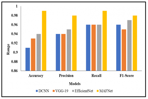
In the analysis of Feature Extraction using MAFNet from Table 2, DCNN has 0.91 ACC, PR level, F1 of 0.96 and 0.96 of RC.VGG-19 has ACC rate of 0.93, RC of 0.96, PR of 0.94, and F1 of 0.95. EfficientNet attained the ACC level of 0.94, PR of 0.95, F1 of 0.97, RC of 0.96 and the MAFNet has 0.99 of ACC, F1 of 0.98, PR of 0.98, RC of 0.99. When comparing with all other models, MAFNet achieved better performance in ACC analysis with 0.99. Figure 8 offering the graphical description of proposed model.
Figure 8. Analysis of feature extraction using MAFNet
4.4 Analysis of classification with existing models
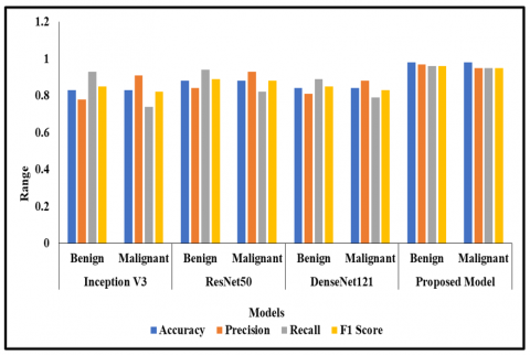
The existing techniques which are DenseNet121, ResNet50, Inception V3 are used for analysis of feature classification. The performance metrices include ACC, RC, F1 and PR were taken to teste the existing models with the proposed model.
From Table 3, the analysis of Inception V3 model benign and malignant have ACC 0.83. In REsNet50, both achieved ACC level 0.88. In DenseNet121 model analysis, both benign and malignant have ACC level 0.84. In proposed technique, both have an ACC level 0.98. Inception V3, benign has a PR of 0.78, 0.85 of F1 and 0.93 of RC. In the analysis of ResNet50 model, benign has a PR of 0.84, 0.89 of F1 and 0.94 of RC. In the analysis of DenseNet121 model, benign has a PR of 0.81, 0.85 of F1 and 0.89 of RC. In the analysis of the proposed model, benign has a PR of 0.97, 0.96 of F1 and 0.96 of RC. Inception V3, malignant has a PR of 0.91, 0.82 of F1 and 0.74 of RC. In the analysis of ResNet50 model, malignant has a PR of 0.93, 0.88 of F1 and 0.82 of RC. In the analysis of DenseNet121 model, malignant has a PR of 0.88, 0.83 of F1 and 0.79 of RC. In the analysis of the proposed model, malignant has a PR of 0.96, 0.95 of F1 and 0.96 of RC. When comparing with all other models, the proposed model achieved better performance in ACC analysis with 0.98. The graphical description for Table 3 is represented in Figure 9.
Table 3. Analysis of feature classification
|
Model |
Class |
ACC |
PR |
RC |
F1 |
|
Inception V3 |
Benign Malignant |
0.83 |
0.78 0.91 |
0.93 0.74 |
0.85 0.82 |
|
ResNet50 |
Benign Malignant |
0.88 |
0.84 0.93 |
0.94 0.82 |
0.89 0.88 |
|
DenseNet121 |
Benign Malignant |
0.84 |
0.81 0.88 |
0.89 0.79 |
0.85 0.83 |
|
Proposed Model |
Benign Malignant |
0.98
|
0.97 0.96 |
0.96 0.96 |
0.96 0.95 |
Figure 9. Analysis of feature classification
Table 4. Analysis of hybrid optimization based on ACO-RSA
|
Existing Techniques |
Without Optimization |
With Optimization |
||||||
|
|
ACC |
PR |
RC |
F1 |
ACC |
PR |
RC |
F1 |
|
InceptionV3 |
85 |
87 |
84 |
86 |
89 |
89 |
85 |
88 |
|
ResNet50 |
87 |
84 |
78 |
87 |
88 |
86 |
79 |
89 |
|
DenseNet121 |
85 |
79 |
86 |
87 |
89 |
83 |
91 |
89 |
|
Proposed Model |
95 |
94 |
95 |
94 |
98 |
97 |
97 |
98 |
Figure 10. Analysis of hybrid optimization based on ACO-RSA
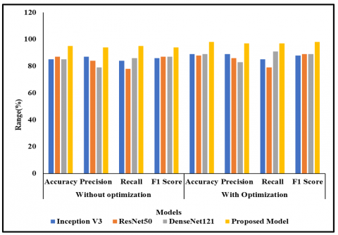
In the analysis of existing techniques without hybrid optimization from Table 4, Inception V3 has 85% ACC, 87% of PR, 86% of F1 and 84% of RC. ResNet50 has ACC rate 87%, RC 78%, F1 level 87% and PR level of 84%. DenseNet121 has ACC level 85%, RC of 86%, PR level of 79%, and F1 87%. On analysing the proposed model, it has 95% of ACC, PR the same as ACC level 95%, F1 level 94% and RC level 95%. In the analysis of existing techniques with optimization, Inception V3 has 89% ACC 89% of PR, 88% of F1 and 85% of RC. ResNet50 has ACC rate of 88%, RC of 79%, PR of 86%, and then F1 of 89%. DenseNet121 has an ACC level of 89%, F1 level 89%, PR 83% and RC 91% and F1 of 89%. On analysing the proposed model with optimization, it has 98% of ACC, 97% PR, 97% RC, 98% F1. When comparing with all other models, the proposed model achieved better performance in ACC analysis with 98%. Figure 10 offering the graphical description of proposed model. The hyperparameters are tuned using hybrid optimization in the proposed model. Hence the proposed model achieves better ACC than the existing techniques.
Mammogram pictures are categorized into four groups in this research utilizing the CBIS-DDSM dataset and the proposed approach. Noise is removed in this case using an image pre-processing approach. To further enhance the quality of the unprocessed mammography, backdrop elimination and methods for enhancing images were employed. The feature of extraction employs the MAFNet model. The learning rate indicated in MAFNet is optimized using the SMO approach. Following feature extraction, feature categorization is carried out by using the AlexNet model. In this work, hybrid optimization in the form of ACO-RSA is used to fine-tune the hyperparameters in feature classification based on AlexNet. As a consequence, the suggested system's performance metrics evaluation revealed that it had a 98% accuracy rate, which is a superior outcome than other current models. Future image fusion approaches will integrate the tumor segmentation phase, and segmentation taken into consideration for the process feature extraction. The computational time issue will be addressed by an improved feature fusion method.
[1] Dang, L.M., Piran, M.J., Han, D., Min, K., Moon, H. (2019). A survey on internet of things and cloud computing for healthcare. Electronics, 8(7): 768. https://doi.org/10.3390/electronics8070768
[2] Chehri, A., Mouftah, H.T. (2020). Internet of Things-integrated IR-UWB technology for healthcare applications. Concurrent Computing: Practice and Experience, 32: e5454. https://doi.org/10.1002/cpe.5454
[3] Chandy, A. (2019). A review on IoT based medical imaging technology for healthcare applications. Journal of Innovative Image Processing, 1: 51-60. https://doi.org/10.36548/jiip.2019.1.006
[4] Karthick, G.S., Pankajavalli, P.B. (2020). A review on human healthcare internet of things: A technical perspective. SN Computer Science, 1: 198. https://doi.org/10.1007/s42979-020-00205-z
[5] Rao, M.V., Sreeraman, Y., Mantena, S.V., Gundu, V., Roja, D., Vatambeti, R. (2024). Brinjal crop yield prediction using shuffled shepherd optimization algorithm based ACNN-OBDLSTM model in Smart Agriculture. Journal of Integrated Science and Technology, 12(1): 710-710.
[6] Pati, A., Parhi, M., Pattanayak, B.K., Sahu, B., Khasim, S. (2023). CanDiag: Fog empowered transfer deep learning based approach for cancer diagnosis. Designs, 7(3): 57. https://doi.org/10.3390/designs7030057
[7] Mann, R.M., Athanasiou, A., Baltzer, P.A.T., et al. (2022). Breast cancer screening in women with extremely dense breasts recommendations of the European Society of Breast Imaging (EUSOBI). European Radiology, 32: 4036-4051. https://doi.org/10.1007/s00330-022-08617-6
[8] Jagadesh, B.N., Karthik, M.G., Siri, D., Shareef, S.K.K., Mantena, S.V., Vatambeti, R. (2023). Segmentation using the IC2T model and classification of diabetic retinopathy using the rock hyrax swarm-based coordination attention mechanism. IEEE Access, 11: 124441-124458. https://doi.org/10.1109/ACCESS.2023.3330436
[9] Yadavendra, Chand, S. (2020). A comparative study of breast cancer tumor classification by classical machine learning methods and deep learning method. Machine Vision and Applications, 31(6): 46. https://doi.org/10.1007/s00138-020-01094-1
[10] Sunardi, Yudhana, A., Putri, A.R.W. (2023). Optimization of breast cancer classification using faster R-CNN. Revue d'Intelligence Artificielle, 37(1): 39-45. https://doi.org/10.18280/ria.370106
[11] Li, H., Niu, J., Li, D., Zhang, C. (2021). Classification of breast mass in two-view mammograms via deep learning. IET Image Processing, 15: 454-467. https://doi.org/10.1049/ipr2.12035
[12] Hanon, W., Salman, M.A. (2024). Integration of ML techniques for early detection of breast cancer: Dimensionality reduction approach. Ingénierie des Systèmes d’Information, 29(1): 347-353. https://doi.org/10.18280/isi.290134
[13] AlSawaftah, N., El-Abed, S., Dhou, S., Zakaria, A. (2022). Microwave imaging for early breast cancer detection: Current state, challenges, and future directions. Journal of Imaging, 8: 123. https://doi.org/10.3390/jimaging8050123
[14] Wang, X., Liang, G., Zhang, Y., Blanton, H., Bessinger, Z., Jacobs, N (2020). Inconsistent performance of deep learning models on mammogram classification. Journal of the American College of Radiology, 17(6): 796–803. https://doi.org/10.1016/j.jacr.2020.01.006
[15] Pati, A., Parhi, M., Pattanayak, B.K., Singh, D., Singh, V., Kadry, S., Nam, Y., Kang, B.G. (2023). Breast cancer diagnosis based on IoT and deep transfer learning enabled by fog computing. Diagnostics, 13(13): 2191. https://doi.org/10.3390/diagnostics13132191
[16] Rajeswari, R., Sriramakrishnan, G.V., Vidyadhari, C., Kanimozhi, K.V. (2023). ExpHBA Deep-IoT: Exponential honey badger optimized deep learning for breast cancer detection in IoT healthcare system. Journal of Digital Imaging, 36(6): 2461-2479. https://doi.org/10.1007/s10278-023-00878-x
[17] Kwak, D., Choi, J., Lee, S. (2023). Rethinking breast cancer diagnosis through deep learning-based image recognition. Sensors, 23(4): 2307. https://doi.org/10.3390/s23042307
[18] Park, S., Kim, J.H., Cha, Y.K., Chung, M.J., Woo, J.H., Park, S. (2023). Application of machine learning algorithm in predicting axillary lymph node metastasis from breast cancer on preoperative chest CT. Diagnostics, 13(18): 2953. https://doi.org/10.3390/diagnostics13182953
[19] Gao, Y., Rezaeipanah, A. (2023). An ensemble classification method based on deep neural networks for breast cancer diagnosis. Inteligencia Artificial, 26(72): 160-177.
[20] Ali, M.D., Saleem, A., Elahi, H., Khan, M.A., Khan, M.I., Yaqoob, M.M., Farooq Khattak, U., Al-Rasheed, A. (2023). Breast cancer classification through meta-learning ensemble technique using convolution neural networks. Diagnostics, 13(13): 2242. https://doi.org/10.3390/diagnostics13132242
[21] Thirumalaisamy, S., Thangavilou, K., Rajadurai, H., Saidani, O., Alturki, N., Mathivanan, S.K., Jayagopal, P., Gochhait, S. (2023). Breast cancer classification using synthesized deep learning model with metaheuristic optimization algorithm. Diagnostics, 13(18): 2925. https://doi.org/10.3390/diagnostics13182925
[22] Liu, C.H., Yang, J.H., Liu, Y., Zhang, Y., Liu, S., Chaikovska, T., Liu, C. (2023). Artificial intelligence in cervical cancer research and applications. Acadlore Transactions on Machine Learning, 2(2): 99-115. https://doi.org/10.56578/ataiml020205
[23] Beeravolu, A.R., Azam, S., Jonkman, M., Shanmugam, B., Kannoorpatti, K., Anwar, A. (2021). Preprocessing of breast cancer images to create datasets for Deep-CNN. IEEE Access, 9: 33438-33463. https://doi.org/10.1109/ACCESS.2021.3058773
[24] Wang, Z., Li, M., Wang, H., Jiang, H., Yao, Y., Zhang, H., Xin, J. (2019). Breast cancer detection using extreme learning machine based on feature fusion with CNN deep features. IEEE Access, 7: 105146-105158. https://doi.org/10.1109/ACCESS.2019.2892795
[25] Dhar, P. (2021). A method to detect breast cancer based on morphological operation. International Journal of Education and Management Engineering, 11: 25-31. https://doi.org/10.5815/ijeme.2021.02.03
[26] Hassan, N., Ullah, S., Bhatti, N., Mahmood, H., Zia, M. (2021). The retinex based improved underwater image enhancement. Multimedia Tools and Applications, 80: 1839-1857. https://doi.org/10.1007/s11042-020-09752-2
[27] Vatambeti, R., Damera, V.K. (2023). Intelligent diagnosis of obstetric diseases using HGS-AOA based extreme learning machine. Acadlore Transactions on Machine Learning, 2(1): 21-32. https://doi.org/10.56578/ataiml020103
[28] Xu, H., Jin, L., Shen, T., Huang, F. (2021). Skin cancer diagnosis based on improved multiattention convolutional neural network. In 2021 IEEE 5th Advanced Information Technology, Electronic and Automation Control Conference (IAEAC), Chongqing, China, 5: 761-765. https://doi.org/10.1109/IAEAC50856.2021.9390972
[29] Kadampur, M.A., Al Riyaee, S. (2020). Skin cancer detection: Applying a deep learning-based model driven architecture in the cloud for classifying dermal cell images. Informatics in Medicine Unlocked, 18: 100282. https://doi.org/10.1016/j.imu.2019.100282
[30] Reddy, N.V.R.S., Chitteti, C., Yesupadam, S., Desanamukula, V.S., Vellela, S.S., Bommagani, N.J. (2023). Enhanced speckle noise reduction in breast cancer ultrasound imagery using a hybrid deep learning model. Ingénierie des Systèmes d’Information, 28(4): 1063-1071. https://doi.org/10.18280/isi.280426
[31] Gupta, P., Garg, S. (2020). Breast cancer prediction using varying parameters of machine learning models. Procedia Computer Science, 171: 593-601. https://doi.org/10.1016/j.procs.2020.04.064
[32] Chen, J., Han, J., Liu, C., Wang, Y., Shen, H., Li, L. (2022). A deep-learning method for the classification of apple varieties via leaf images from different growth periods in a natural environment. Symmetry, 14(8): 1671. https://doi.org/10.3390/sym14081671
[33] Das, A., Mohanty, M.N., Mallick, P.K., Tiwari, P., Muhammad, K., Zhu, H. (2021). Breast cancer detection using an ensemble deep learning method. Biomedical Signal Processing and Control, 70: 103009. https://doi.org/10.1016/j.bspc.2021.103009
[34] Kumar, S., Sharma, B., Sharma, V.K., Sharma, H., Bansal, J.C. (2020). Plant leaf disease identification using exponential spider monkey optimization. Sustainable Computing: Informatics and Systems, 28: 100283. https://doi.org/10.1016/j.suscom.2018.10.004
[35] Kumar, S., Sharma, B., Sharma, V.K., Poonia, R.C. (2021). Automated soil prediction using bag-of-features and chaotic spider monkey optimization algorithm. Evolutionary intelligence, 14: 293-304. https://doi.org/10.1007/s12065-018-0186-9
[36] Wu, Y., Gong, M., Ma, W., Wang, S. (2019). High-order graph matching based on ant colony optimization. Neurocomputing, 328: 97-104. https://doi.org/10.1016/j.neucom.2018.02.104
[37] Shayma’a, A.H., Sayed, M.S., Abdalla, M.I.I., Rashwan, M.A. (2020). Breast cancer masses classification using deep convolutional neural networks and transfer learning. Multimedia Tools and Applications, 79: 30735-30768. https://doi.org/10.1007/s11042-020-09518-w