OPEN ACCESS
This paper presents the design of a new nonlinear control for the doubly fed induction machine (DFIM). The proposed control is based on a Backstepping type control technique supplemented by a type 1 fuzzy controller to improve its robustness. Using the Lyapunov stability theory, it is shown that trajectory tracking dynamics are asymptotically stable. In order to simplify the control, we apply the control by orientation of the stator flux which has the advantage of having a decoupling between the flow and the current. The simulation results show the quality of the proposed control despite parametric uncertainties
doubly-fed induction machine (DFIM), backstepping control, theory of lyapunov, stator flux orientation, fuzzy logic, hybrid control, robustness
The control of nonlinear systems was of great interest at the end of the 1980s, with the first version of input-output linearization. (Krstie and Kokotovie, 1995; Kokotovie, 1992), introduced methods using recursive variable changes called backstepping, on classes of parametric nonlinear triangular systems. In general, the proposed control laws satisfy good properties of robustness and attenuation of disturbances, but only apply to restricted classes of systems and use only static controllers. By introducing a dynamic change of variables and using a Lyapunov function, simple controllers and adaptation laws were obtained for more general classes of nonlinear systems in 1980 (Marce et al., 1981).
Among the non-linear systems most used in the world of industry is the dual-power asynchronous machine, it is a three-phase asynchronous machine with a wound rotor that can be powered by two voltage sources, one to the stator and the other to the rotor (Vicatos et al., 2003; Rouabhi, 2016). This is due to several factors such as: the quality of robustness, reliability where we mainly appreciate its low maintenance and low cost and very good standardization. The absence of natural decoupling between the inductor and the armature, gives the dual-power asynchronous machine a non-linear dynamic model which is the opposite of the simplicity of its structure. Therefore, his order poses a theoretical problem which complicates his model because the parameters of the asynchronous dual feed machine are known approximately and can vary with time (temperature), hence the interest of using the command robust by backstepping.
The backstepping technique has been applied for various electric motors, in particular the doubly-fed induction motor (Fadili et al., 2013; Tan et al., 1999; Ghanes et al., 2004). This approach consists in finding a Lyapunov function that allows deducing a control law for the system while showing the overall control stability. On the other hand, the vector control of the asynchronous machine aims to match the performance offered by the control of a separate excitation DC machine. Indeed, in the latter the decoupling between the flux and the torque is naturally achieved which makes these two quantities independently controlled (Ghanes, 2004).
This work presents the application of the backstepping to the control of the doubly-fed induction machine, based on the principle of the orientation of the stator flux. This approach allows us to determine the components of the machine supply voltages by ensuring the overall stability by Lyapunov's theory. The control thus obtained makes it possible to monitor speed, flux and current, each time ensuring stable dynamics for errors between the reference and actual quantities of speed, flux and current.
In the end, we propose a command based on backstepping and type 1 fuzzy logic to build iteratively and systematically an asymptotically stable robust control law according to the Lyapunov stability theory. This technique consists in replacing the gains of the regulations in the backstepping command by a fuzzy controller of type 1 at an input are the error between the measured value and the reference value. The proposed control technique presents high performance transient and permanent and also vis-à-vis parametric uncertainties.
The rest of this article is organized as follows. Section 2 recalls the mathematical model of the DFIM and the simplified model which has a decoupling between the flow and the current. In the 3 section, we synthesize a backstepping control law of the DFIM. Then section fourth presents a theoretical study on fuzzy logic type 1. Simulation results are presented in the fifth section and conclusions are drawn in the last part of this article.
The model of the doubly-fed induction machine is expressed in a reference linked to the rotating field (d,q), the electrical equations of the DFIM write in the form:
$\left\{ \begin{array} { l } { V _ { s d } = R _ { s } I _ { s d } + \frac { d \varphi _ { s d } } { d t } - \omega _ { s } \varphi _ { s q } } \\ { V _ { s q } = R _ { s } I _ { s q } + \frac { d \varphi _ { s q } } { d t } + \omega _ { s } \varphi _ { s d } } \\ { V _ { r d } = R _ { r } I _ { r d } + \frac { d \varphi _ { r d } } { d t } - \left( \omega _ { s } - \omega _ { r } \right) \varphi _ { r q } } \\ { V _ { r q } = R _ { r } I _ { r q } + \frac { d \varphi _ { r q } } { d t } + \left( \omega _ { s } - \omega _ { r } \right) \varphi _ { r d } } \end{array} \right.$ (1)
Where:
$\omega _ { r } = \omega _ { s } - P . \Omega$
The magnetic equations of the DFIM can be written:
$\left\{ \begin{array} { l } { \varphi _ { s d } = L _ { s } I _ { s d } + M \cdot I _ { r d } } \\ { \varphi _ { s q } = L _ { s } I _ { s d } + M \cdot I _ { r q } } \\ { \varphi _ { r d } = L _ { r } I _ { r d } + M \cdot I _ { s d } } \\ { \varphi _ { r q } = L _ { r } I _ { r q } + M \cdot I _ { s q } } \end{array} \right.$ (2)
$L _ { s } = l _ { s } - M _ { s }$ and $L _ { r } = l _ { r } - M _ { r }$ cyclic inductances of a stator and rotor phase;
$\left[ l _ { s } \right]$ and $\left[ l _ { r } \right]$ own inductances of a stator and rotor phase;
$M _ { s }$ and $M _ { r }$ mutual inductances between two phases respectively stator and rotor;
M: maximum mutual inductance between a stator and rotor phase (the axes of the two phases coincide).
The expression of the electromagnetic torque of the DFIM according to the stator flows and currents is written as follows:
$C _ { e m } = P \frac { M } { L _ { s } } \left( \varphi _ { s q } I _ { r d } - \varphi _ { s d } I _ { r q } \right)$ (3)
With P: number of pairs of DFIM poles.
The model of the doubly-fed induction machine can be written in matrix form as follows (Rouabhi, 2016):
$\dot { X } = A X + B U$ (4)
Where:
$X = \left[ \begin{array} { c c c c } { \varphi _ { s d } } & { \varphi _ { s q } } & { I _ { r d } } & { I _ { r q } } \end{array} \right] ^ { T }$ and $U = \left[ \begin{array} { c c c } { V _ { s d } } & { V _ { s q } } & { V _ { r d } } & {\left. V _ { r q } \right] ^ { T } } \end{array} \right.$ $[ A ] = \left[ \begin{array} { c c c c } { - \frac { 1 } { T _ { S } } } & { \omega _ { S } } & { \frac { M } { T _ { S } } } & { 0 } \\ { - \omega _ { S } } & { - \frac { 1 } { T _ { S } } } & { 0 } & { \frac { M } { T _ { S } } } \\ { \alpha } & { - \beta \omega } & { - \delta } & { \left( \omega _ { S } - \omega \right) } \\ { \beta \omega } & { \alpha } & { - \left( \omega _ { S } - \omega \right) } & { - \delta } \end{array} \right]$; $[ B ] = \left[ \begin{array} { c c c c } { 1 } & { 0 } & { 0 } & { 0 } \\ { 0 } & { 1 } & { 0 } & { 0 } \\ { - \frac { M } { \sigma L _ { s } L _ { r } } } & { 0 } & { \frac { 1 } { \sigma L _ { r } } } & { 0 } \\ { 0 } & { - \frac { M } { \sigma L _ { s } L _ { r } } } & { 0 } & { \frac { 1 } { \sigma L _ { r } } } \end{array} \right]$ With: $\sigma = 1 - \frac { M ^ { 2 } } { L _ { r } L _ { S } } ; $ $T _ { r } = \frac { L _ { r } } { R _ { r } } ; $ $T _ { s } = \frac { L _ { s } } { R _ { s } } ; $ $\alpha = \frac { M } { \sigma L _ { r } L _ { s } T _ { S } } ;$ $ \beta = \frac { M } { \sigma L _ { r } L _ { s } } ; $ $\delta = \frac { 1 } { \sigma } \left( \frac { 1 } { T _ { r } } + \frac { M ^ { 2 } } { L _ { s } T _ { s } L _ { r } } \right)$
The mechanical equation is of the following form:
$J \frac { d \Omega } { d t } = C _ { e m } - C _ { r } - f \Omega$ (5)
With:
$C _ { e m }$ and $C _ { r }$ the electromagnetic torque and the resisting torque (the mechanical load); f and J: coefficient of friction and moment of inertia of the rotor shaft.
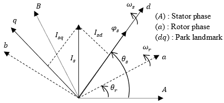
In our study, the frequency and the tension are constant. We can see, from relation (3), the strong coupling between flows and currents. Indeed, the electromagnetic torque is the cross product between the flows and the stator currents, which makes the control of the DFIM particularly difficult. In order to simplify the order, we approximate its model to that of the DC machine which has the advantage of having a natural decoupling between the flows and the currents. For this, we apply the flow orientation control which consists in aligning the stator flux $\varphi _ { S }$ along the d axis of the rotating reference, (Figure 1), (Vidal, 2004; Boyette A., 2006). We thus have: $\varphi _ { Sd }$=$\varphi _ { S }$ and consequently $\varphi _ { S }=0$.
Figure 1. Stator flux orientation on the axis
The electromagnetic torque of equation (3) is then written:
$C _ { e m } = - P \frac { M } { L _ { S } } \varphi _ { S d } I _ { r q }$ (6)
And the equation (2) of the flows becomes:
$\left\{ \begin{array} { l } { \varphi _ { s d } = \varphi _ { s } = L _ { s } I _ { s d } + M \cdot I _ { r d } } \\ { \varphi _ { s q } = 0 = L _ { s } I _ { s q } + M \cdot I _ { r q } } \end{array} \right.$ (7)
$So: \left\{ \begin{array} { l } { I _ { s d } = \frac { 1 } { L _ { s } } \left( \varphi _ { s } - M I _ { r d } \right) } \\ { I _ { s q } = - \frac { 1 } { L _ { s } } M I _ { r q } } \end{array} \right.$
If one takes the stator current in the axis of null, Isd=0, realistic hypothesis for the machines of high power, the current and the tension in this axis are then in phase $V _ { S } = V _ { S q }$ and $I _ { S } = I _ { S q }$.
In this case, we get:
$\left\{ \begin{array} { l } { I _ { r d } = \frac { \varphi _ { s } } { M } } \\ { I _ { r q } = - \frac { L _ { s } } { P M \varphi _ { s } } C _ { e m } } \end{array} \right.$ (8)
With the assumption of constant stator flux, we obtain the electric equations in the form:
$\left\{ \begin{array} { l } { V _ { s d } = R _ { s } I _ { s d } } \\ { V _ { s q } = R _ { s } I _ { s q } + \omega _ { s } \varphi _ { s d } } \\ { V _ { r d } = R _ { r } I _ { r d } - \left( \omega _ { s } - \omega _ { r } \right) \varphi _ { r q } } \\ { V _ { r q } = R _ { r } I _ { r q } + \left( \omega _ { s } - \omega _ { r } \right) \varphi _ { r d } } \end{array} \right.$ (9)
In the principle of the orientation of the stator field ($\varphi _ { s q } = 0$), the model of the doubly-fed induction machine is written:
$\left\{ \begin{array} { l } { \frac { d \varphi _ { s d } } { d t } = \frac { M } { T _ { s } } I _ { r d } - \frac { 1 } { T _ { s } } \varphi _ { s d } + V _ { s d } } \\ { \frac { d \varphi _ { s q } } { d t } = \frac { M } { T _ { s } } I _ { r q } - \omega _ { s } \varphi _ { s d } + V _ { s q } } \\ { \frac { d I _ { r d } } { d t } = - \delta I _ { r d } + \left( \omega _ { s } - \omega \right) I _ { r q } + \alpha \varphi _ { s d } - \frac { M } { \sigma L _ { s } L _ { r } } V _ { s d } + \frac { 1 } { \sigma L _ { r } } V _ { r q } } \\ { \frac { d r q } { d t } = - \left( \omega _ { s } - \omega \right) I _ { r d } - \delta I _ { r q } + \beta \omega \varphi _ { s d } - \frac { M } { \sigma L _ { s } L _ { r } } V _ { s q } + \frac { 1 } { \sigma L _ { r } } V _ { r q } } \end{array} \right.$ (10)
The mechanical equation is written:
$\frac { d \Omega } { d t } = - \frac { 1 } { J } \left( P \frac { M } { L _ { S } } \varphi _ { s d } I _ { r q } + f \Omega + C _ { r } \right)$ (11)
The backstepping control technique is a non-linear synthesis method when it is difficult to apply the direct method of Lyapunov. It is a question of choosing initially a function of Lyapunov for the first subsystem and of increasing it as one stabilizes the various successive subsystems, to finally arrive at a global Lyapunov function which stabilizes the overall system (Tan et al., 1999; Ghanes et al, 2004; Benchaib, 1998).
The backstepping control of the DFIM consists of the following three steps.
Step 1:
This first step consists in identifying the errors z1 and z2 which respectively represent the error between the real speed $\Omega$ and the reference speed $\Omega_{ref}$ as well as the rotor flow modulus $\Omega_{sd}$ and the reference one $\Omega^{ref}_{sd}$.
$\begin{aligned} z _ { 1 } & = \Omega _ { r e f } - \Omega \\ z _ { 2 } & = \varphi _ { s d } ^ { r e f } - \varphi _ { s d } \end{aligned}$ (12)
The derivative of the error is given by:
$\begin{aligned} \dot { z } _ { 1 } & = \dot { \Omega } _ { \text {ref} } - \dot { \Omega } = \dot { \Omega } _ { \text {ref} } + \frac { 1 } { J } \left( P \frac { M } { L _ { s } } \varphi _ { s d } I _ { r q } + f \Omega + C _ { r } \right) \\ \dot { z } _ { 2 } & = \dot { \varphi } _ { s d } ^ { r e f } - \dot { \varphi } _ { s d } = \dot { \varphi } _ { s d } ^ { r e f } - \left( \frac { M } { T _ { s } } I _ { r d } - \frac { 1 } { T _ { s } } \varphi _ { s d } + V _ { s d } \right) \end{aligned}$ (13)
The first function of Lyapunov is defined by:
$v _ { 1 } = \frac { 1 } { 2 } \left( z _ { 1 } ^ { 2 } + z _ { 2 } ^ { 2 } \right)$ (14)
Then, the derivative of (14) is calculated as:
$\dot { v } _ { 1 } = z _ { 1 } \left( \dot { \Omega } _ { r e f } + \frac { 1 } { J } \left( P \frac { M } { L _ { s } } \varphi _ { s d } I _ { r q } + f \Omega + C _ { r } \right) \right) + z _ { 2 } \left( \dot { \varphi } _ { s d } ^ { r e f } - \left( \frac { M } { T _ { s } } I _ { r d } - \frac { 1 } { T _ { s } } \varphi _ { s d } + V _ { s d } \right) \right)$ (15)
The stabilizing functions are chosen as follows:
$\left\{ \begin{array} { l } { I _ { r q } ^ { r e f } = - \frac { J L _ { s } } { p M \varphi _ { s d } } \left( k _ { 1 } z _ { 1 } + \dot { \Omega } _ { r e f } + \frac { f } { J } \Omega + \frac { c _ { r } } { J } \right) } \\ { I _ { r d } ^ { r e f } = \frac { T _ { s } } { M } \left( k _ { 2 } z _ { 2 } + \dot { \varphi } _ { s d } ^ { r e f } - V _ { s d } + \frac { 1 } { T _ { s } } \varphi _ { s d } \right) } \end{array} \right.$ (16)
Where k1 and k2 are positive design constants. Then (13) can be expressed as:
$\begin{aligned} \dot { z } _ { 1 } & = - k _ { 1 } z _ { 1 } \\ \dot { z } _ { 2 } & = - k _ { 2 } z _ { 2 } \end{aligned}$ (17)
The derivative of the function of Lyapunov with respect to time is:
$\dot { v } _ { 1 } = - k _ { 1 } z _ { 1 } ^ { 2 } - k _ { 2 } z _ { 2 } ^ { 2 } < 0$ (18)
Step 2:
In this step, two new errors of the components of the current given by:
$z _ { 3 } = I _ { r q } ^ { r e f } - I _ { r q } = - \frac { J L _ { s } } { p M \varphi _ { s d } } \left( k _ { 1 } z _ { 1 } + u _ { 1 } \right) - I _ { r q }$
$z _ { 4 } = I _ { r d } ^ { r e f } - I _ { r d } = \frac { T _ { s } } { M } \left( k _ { 2 } z _ { 2 } + u _ { 2 } \right) - I _ { r d }$ (19)
Its derivative is given by:
$\begin{aligned} \dot { z } _ { 3 } & = \dot { I } _ { r q } ^ { r e f } - \dot { I } _ { r q } = \dot { I } _ { r q } ^ { r e f } - \left( \eta _ { 1 } + \frac { 1 } { \sigma L _ { r } } V _ { r q } \right) \\ \dot { z } _ { 4 } & = \dot { I } _ { r d } ^ { r e f } - \dot { I } _ { r d } = \dot { I } _ { r d } ^ { r e f } - \left( \eta _ { 2 } + \frac { 1 } { \sigma L _ { r } } V _ { r d } \right) \end{aligned}$ (20)
$Or: \left\{ \begin{array} { l } { \eta _ { 1 } = - \left( \omega _ { s } - \omega \right) I _ { r d } - \delta I _ { r q } + \beta \omega \varphi _ { s d } - \frac { M } { \sigma L _ { s } L _ { r } } V _ { s q } } \\ { \eta _ { 2 } = - \delta I _ { r d } + \left( \omega _ { s } - \omega \right) I _ { r q } + \alpha \varphi _ { s d } - \frac { M } { \sigma L _ { s } L _ { r } } V _ { s d } } \end{array} \right.$
Step 3:
To define the control laws, we adopt a new function of lyapunov described by the following expression:
$v _ { 2 } = \frac { 1 } { 2 } \left( z _ { 1 } ^ { 2 } + z _ { 2 } ^ { 2 } + z _ { 3 } ^ { 2 } + z _ { 4 } ^ { 2 } \right)$ (21)
So, the derivative of the final lyapunov function is:
$\dot { v } _ { 2 } = z _ { 1 } \dot { z } _ { 1 } + z _ { 2 } \dot { z } _ { 2 } + z _ { 3 } \dot { z } _ { 3 } + z _ { 4 } \dot { z } _ { 4 }$ (22)
This equation can be rewritten in the following from:
$\dot { v } _ { 2 } = z _ { 1 } \dot { z } _ { 1 } + z _ { 2 } \dot { z } _ { 2 } + z _ { 3 } \left( k _ { 3 } z _ { 3 } + \dot { I } _ { r q } ^ { r e f } - \eta _ { 1 } - \frac { 1 } { \sigma L _ { r } } V _ { r q } \right) + z _ { 4 } \left( k _ { 4 } z _ { 4 } + \dot { I } _ { r d } ^ { r e f } - \eta _ { 2 } - \frac { 1 } { \sigma L _ { r } } V _ { r d } \right)$ (23)
We choose the command as follows:
$\begin{aligned} V _ { r q } ^ { r e f } & = \sigma L _ { r } \left( k _ { 3 } z _ { 3 } + \dot { I } _ { r q } ^ { r e f } - \eta _ { 1 } \right) \\ V _ { r d } ^ { r e f } & = \sigma L _ { r } \left( k _ { 4 } z _ { 4 } + \dot { I } _ { r d } ^ { r e f } - \eta _ { 2 } \right) \end{aligned}$ (24)
The choice of $k _ { 3 } > 0$ and $k _ { 4 } > 0$ can be made such that $\dot { v } _ { 2 } < 0$.
Then, (20) can be expressed as:
$\begin{aligned} \dot { z } _ { 3 } & = - k _ { 3 } z _ { 3 } \\ \dot { z } _ { 4 } & = - k _ { 4 } z _ { 4 } \end{aligned}$ (25)
So, from equation (17) and (25) we can write:
$\dot { v } _ { 2 } = - k _ { 1 } z _ { 1 } ^ { 2 } - k _ { 2 } z _ { 2 } ^ { 2 } - k _ { 3 } z _ { 3 } ^ { 2 } - k _ { 4 } z _ { 4 } ^ { 2 } < 0$ (26)
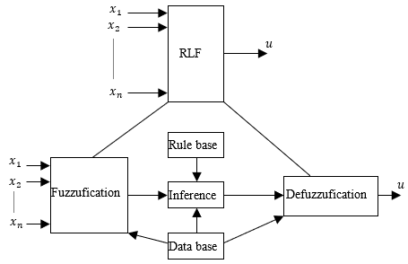
The structure of a complete fuzzy control system is composed from the following blocs: Fuzzification, Knowledge base, Inference engine, Defuzzification. Figure 2 shows the structure of a fuzzy logic controller.
Figure 2. The structure of a fuzzy logic controller
The fuzzification module converts the crisp values of the control inputs into fuzzy values. A fuzzy variable has values, which are defined by linguistic variables (fuzzy sets or subsets) such as low, medium, high, slow… where each is defined by gradually varying membership function. In fuzzy set terminology, all the possible values that a variable can assume are named universe of discourse, and fuzzy sets (characterized by membership function) cover whole universe of discourse. The shape fuzzy sets can be triangular, trapezoidal, etc. (Aissaoui et al., 2007).
A fuzzy control essentially embeds the intuition and experience of a human operator, and sometimes those of a designer and researcher. The data base and the rules form the knowledge base which is used to obtain the inference relation R. The data base contains a description of input and output variables using fuzzy sets. The rule base is essentially the control strategy of the system. It is usually obtained from expert knowledge or heuristics; it contains a collection of fuzzy conditional statements expressed as a set of IF-THEN rules, such as:
$R ^ { ( i ) } :$ If $x _ { 1 }$ is $F _ { 1 }$ and $x _ { 2 }$ is $F _ { 2 } \ldots$ and $x _ { n }$ is $F _ { n }$
Then $Y$ is $G ^ { ( i ) } , i = 1 , \ldots , M$ (27)
Where: $\left( x _ { 1 } , x _ { 2 } , \dots , x _ { n } \right)$ is the input variables vector, Y is the control variable, M is the number of rules, n is the number fuzzy variables, $\left( F _ { 1 } , F _ { 2 } , \ldots F _ { n } \right)$ are the fuzzy sets.
For the given rule base of a control system, the fuzzy controller determines the rule base to be fired for the specific input signal condition and then computes the effective control action (the output fuzzy variable) (Aissaoui et al., 2007; Ben et al., 2010).
The composition operation is the method by which such a control output can be generated using the rule base. Several composition methods, such as max-min or sup-min and max-dot have been proposed in the literature.
The mathematical procedure of converting fuzzy values into crisp values is known as “defuzzification”. A number of defuzzification methods have been suggested. The choice of defuzzification methods usually depends on the application and the available processing power. This operation can be performed by several methods of which center of gravity (or centroid) and height methods are common (Aissaoui et al., 2007; Ben et al., 2010).
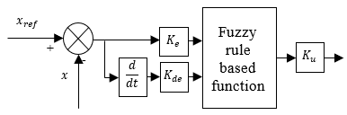
The supervisory type-1 fuzzy of the proposed tuning method contains operator’s knowledge in the form IF-THEN rules decide the control gains Ki according to the current operating condition of the controlled system. Here, the control rules of the supervisory fuzzy system are developed with the error e and derivative of error e as the premise. And $K _ { i } , i = 1 , \dots , 4$ as a consequent of each rules (Amer et al., 2011; Zeghlache et al., 2017).
The general structure of the proposed controller is given in Figure 3.
Figure 3. Block diagram of Fuzzy controller
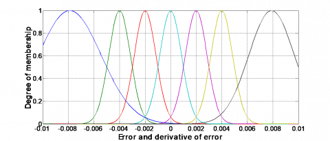
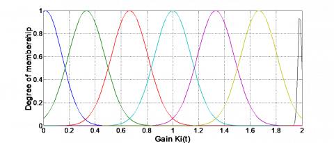
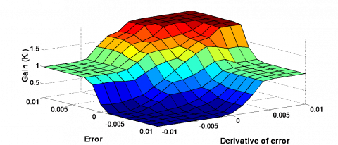
The membership functions for the inputs and outputs as shown respectively in Fig. 4 and Fig. 5. Fig. 6 shows the type-1 fuzzy control surface of Ki. This surface has been used to adaptively tune $K _ { i } , i = 1 , \dots , 4$ on line. The physical domain of the inputs $( e , \dot { e } )$ is in the range {-0.01, 0.01} and that of the output Ki is in the range {0, 2}, respectively, selected based on trial and error approach. The fuzzy variables are defined for the rule base as, $( e , \dot { e } )$={NB (Negative Big), NM (Negative Medium), NS (Negative Small), ZE (Zero), PS (Positive Small), PM (Positive Medium), PB (Positive Big)}; Ki= {VVS (Very Very Small), VS (Very Small), S (Small), M (Medium), B (Big), VB (Very Big) and VVB (Very Very Big) }. The linguistic fuzzy rules of the supervisory type-1 fuzzy system is given in Table 1.
Table 1. Rule matrix of supervisory type-1 fuzzy control
|
Ki |
e(t) |
|||||||
|
NB |
NM |
NS |
ZE |
PS |
PM |
PB |
||
|
$\dot{e}(t)$ |
NB |
VVS |
VVS |
VVS |
VVS |
M |
M |
M |
|
NM |
VVS |
VVS |
VS |
VS |
M |
M |
M |
|
|
NS |
VVS |
VVS |
S |
S |
B |
B |
VB |
|
|
ZE |
VVS |
VS |
S |
M |
B |
VB |
VVB |
|
|
PS |
VS |
S |
S |
B |
B |
VVB |
VVB |
|
|
PM |
M |
M |
M |
VB |
VB |
VVB |
VVB |
|
|
PB |
M |
M |
M |
VVB |
VVB |
VVB |
VVB |
|
Figure 4. Membership functions for input $t ( \dot { e } )$
Figure 5. Membership functions for output $K _ { i } ( t )$
Figure 6. Type-1 fuzzy control of Ki
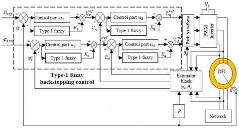
The block diagram of the proposed type-1 fuzzy backstepping control scheme is presented in figure 7. The first step of the command is to generate the currents of $I _ { r q } ^ { r e f }$ and $I _ { r d } ^ { r e f }$, representing the dummy command. The error between these references and the real quantities of the currents results from new errors z3 and z4. Finally, we adapt the control law $V _ { r q } ^ { r e f }$ and $V_ { r d } ^ { r e f }$ from equation (24) to ensure the stability of the machine.
Figure 7. Block diagram of the backstepping control based on fuzzy controller of the DFIM
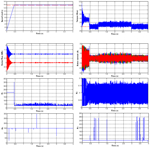
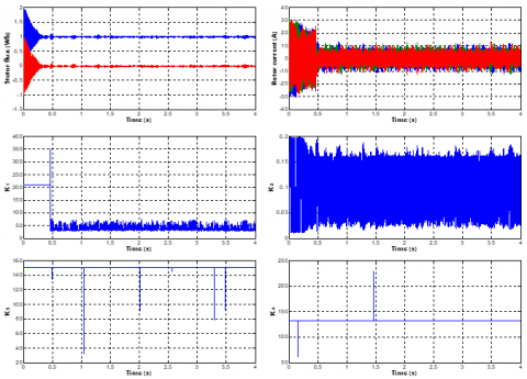
Figure 8. Simulation results of the DFIM controlled by type-1 fuzzy backstepping control
In the second test a load of value Cr=10N. m is applied and between instants t=1s and t=3s a variation on the rotor resistance at (+50%). The variation of the rotor resistance does not affect the speed and flux quantities. The principle of vector control is always verified.
Figure 9. Simulation results of backstepping control of the DFIM based on fuzzy controller with rotor resistance variation (+50%)
This paper presents the robust control of the doubly fed induction machine that is based on backstepping control and type 1 fuzzy controller. In this control we have chosen the gains of the regulation by the type 1 fuzzy. After presenting a Mathematical modeling of DFIM, we applied the orientation of stator flux to have the decoupling between the flux and the current for simplified the model of DFIM.
The interest of this command is the robustness; it is to eliminate the effects of the parametric variations even in dynamic regime with a minimum of complexity of the law of control. The structure of this approach is cascaded by backstepping control and fuzzy logic type 1. Simulations results have then shown robustness and good performances when the DFIM is confronted to internal and external perturbations. Furthermore, this regulation presents a simple robust control algorithm.
Aissaoui M., Abid H., Abid A., Tahour A. (2007). A fuzzy logic controller for synchronous machine. Journal of Electrical Engineering, Vol. 58, No. 5, pp. 285-290. http://iris.elf.stuba.sk/cgi-bin/jeeec?act=pr&no=5_107
Amer A., Sallam E., Elawady W. (2011). Adaptive fuzzy sliding mode control using supervisory fuzzy control for 3 DOF planar robot manipulators. Applied Soft Computing. Vol. 11, pp. 4943-4953. http://dx.doi.org/10.1016/j.asoc.2011.06.005
Ben A. D., Bekakra Y. (2010). Speed control of a doubly fed induction motor using fuzzy logic techniques. International Journal on Electrical Engineering and Informatics, Vol. 2, No. 3, pp. 179-191. http://www.ijeei.org/archives-number-5.html
Benchaib A. (1998). Application des modes de glissement pour la commande en temps réel de la machine asynchrone. Doct. Thesis, University of Picardie Jules Vernes.
Boyette A. (2006). Contrôle-commande d’un générateur asynchrone à double alimentation avec système de stockage pour la production éolienne. Doct. Thesis, Dept. of Elect. Eng., University of Henri Poincaré, Nancy I, France.
Elfadili A., Giri F., El Magri A., Dugard L. (2013). Backstepping controller for doubly fed induction motor with BI-DIRectional AC/DC/AC converte. Preprint submitted to 11th IFAC International Workshop on Adaptation and Learning in Control and Signal Processing. https://hal.archives-ouvertes.fr/hal-00818419/
Ghanes M. (2005). Observation et commande de la machine asynchrone sans capteur de mécanique. Doct. Thesis, université de Nantes. https://tel.archives-ouvertes.fr/tel-00117094/
Ghanes M., Glumineau A., Deleon J. (2004). Backstepping observer validation for sensorless induction motor on low frequencies benchmark. IEEE International Conference on Industrial Technology (ICIT). http://doi.org/10.1109/ICIT.2004.1490760
Kokotovie P. V. (1992). The joy of feedback: Nonlinear and adaptive. IEEE Control Systems Magazine, Vol. 12, pp. 7-17. http://doi.org/10.1109/37.165507
Krstie M., Kokotovie P. V. (1995). Nonlinear and adaptive control design. Proceeding of New York. Wiley.
Marce L., Juliere M., Place H. (1981). Stratégie de contournement d’obstacles pour un robot mobil, Rairo, Vol. 15, No. 1.
Rouabhi R. (2016). Contrôle des puissances générées par un système éolien à vitesse variable basé sur une machine asynchrone double alimentée. Doct. Thesis, Dept. of Elect, university of Batna, Algeria.
Tan H., Chang J. (1999). Adaptative backstepping control of induction motor with uncertainties. Proceedings of the American Control Conference, San diego, California. http://doi.org/10.1109/ACC.1999.782729
Vicatos M. S., Tegopoulos J. A. (2003). A doubly-fed induction machine differential drive model for automobiles. IEEE Trans. Ene. Conv. Vol. 18, No. 2, pp. 225-230. http://doi.org/10.1109/TEC.2003.811732
Vidal P. E. (2004). Commande non-linéaire d'une machine asynchrone à double alimentation. Doct. Thesis, Dept. of Elect. Eng., Institut National Polytechnique de Toulouse, France. http://ethesis.inp-toulouse.fr/archive/00000031/
Zeghlache S., Ghellab M. Z., Bouguerra A. (2017). Adaptive type-2 fuzzy sliding mode control using supervisory type-2 fuzzy control for 6 DOF octorotor aircraft. International Journal of Intelligent Engineering and Systems, Vol. 10, No. 3, pp. 47-57. http://doi.org/10.1007/s11704-015-4448-8