Mourad Jebli* | Thierry Martire | Jean-Charles Laurentie | Guillaume Pellecuer | Ludovic Boyer | Jérôme Castellon
© 2022 IIETA. This article is published by IIETA and is licensed under the CC BY 4.0 license (http://creativecommons.org/licenses/by/4.0/).
OPEN ACCESS
One of the main issues on high voltage direct current (HVDC) cable is the electric field distribution on the insulation induced by space charges accumulation. Indeed, the space charges can cause a local increase of the electric field, which will accelerate ageing and may lead to dielectric breakdown. The TSM is one of the techniques that allow space charge measurements. The principle of the TSM consists in disturbing the electrostatic balance of the cable insulation system using a short thermal stimulus. For this study, the thermal pulse is created by Joule effect. This paper describes the structural optimization of a multi-cell DC-DC converter and its use in a high-current application to produce thermal stimulus. The design of the converter is first presented, then a multi-objective optimization is proposed for minimizing volume and losses. Finally, experimental results using a converter prototype which confirmed the space charge measurement principle are presented.
thermal step method, space charge, multicellular buck converter, magnetic coupler, cyclic cascade, DC/DC converter, non-intrusive measurement, DC cable
High voltage direct current (HVDC) transmission on the last decades emerged as a viable solution for certain transmission applications resulting an increase of HVDC projects commited or under review. HVDC makes it possible to transport the electrical energy on long distances, since the direct current transmission eliminates power losses related to frequency effects. Therefore, the HVDC power transmission can be used to build large electric network with improved stability and lower losses. In this technology, the transmission of electric energy is carried out using HVDC cables which must be highly reliable to improve power availability.
HVDC allows interconnecting power sources of different type like off shore renewable electricity stations, AC power plants, wind turbines and solar plants. Moreover, HVDC is recognized for interconnecting asynchrounus grids where there are different frequencies to interconnect.
In normal use, the insulation of HVDC cables is subjected to two combined stresses that accelerate their ageing. Strong electric field imposed by the transmission high voltage and strong thermal gradients due to Joule effect on the conductor. As a result, space charges appear in the volume of the insulation and induce electric field distortions [1, 2]. The space charges accumulation can lead to dielectric breakdown causing the interruption of energy transmission. The space charge measurement and monitoring over time is one way to assess the electrical state of the insulation and to anticipate possible failures [1, 2].
The quantification and the localization of the space charge is based on disturbing the electrostatic balance of the insulation system between the two electrodes using an excitation (thermal, mechanical, electrical, ...). Then, the reorganization of influence charges in the external circuit induces a response representative of the space charge trapped in the cable insulation [3-5]. In this paper, we focus on a non-destructive and non-intrusive variant of the Thermal Step Method (TSM) that allows the electrical state of the dielectric to be preserved during measurement without machining the cable, respectively.
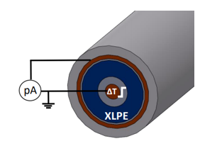
This method is based on the application of a thermal stimulus followed by the measurement of the thermal step current (TS) (Eq. 1) which is representative of the space charge distribution (Figure 1). The digital processing of the measured current makes it possible to calculate the electric field and to deduce the distribution of space charge [1, 2].
$I_{T S}(t)=-\alpha C \int_{R_i}^{R_o} E(r) \frac{d \Delta T}{d t} d r$ (1)
Figure 1. TS current measurement in a power cable using the thermal step method
To measure space charges on long cables, it is necessary to apply the stimulus on the entire length of the cable and then to measure the response of the whole cable. Until now, Joule effects was obtained by injecting an AC 50 Hz heating current into the conductive core of the cable [6, 7] which respects the conditions needed for measurement on long cables. This technique needs a heavy power transformer which absorbs a very high reactive power when the cable length increases.
The TSM principle using AC current can be realized using a transformer [1, 5, 8]. In this configuration, the cable is short circuited and constitutes the secondary of the transformer in which the AC heating current circulates [8]. The heating current can be controlled by adjusting the number of turns on the primary circuit or the applied voltage. However, the TSM using AC current only allows measurements on short cable length (few meters) since this configuration requires high apparent power to compensate the reactive power. The use of DC heating current allows to overcome the drawbacks of AC transformer technique. In this paper, we introduce a new DC heating method using a high current DC/DC converter between the energy source and the cable. First, the power pulse needed to apply the TSM on the reduced cable scale is deduced using numerical simulation. Then, DC converter with optimized design parameters is developed taking into account the needed power pulse specifications. After converter development, a different control system is tested in order to optimize the output current dynamic and to reach the reference output current.
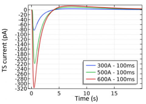
The second step investigates space charge measurements performed for multiple power pulses (250, 350 et 550 A) during short duration (<120 ms). The comparison of TS currents obtained using multiple power pulses is done to prove the measurement principle.
The simulations of the TSM using a DC heating current on a reduced scale cable (Table 1) will provide indications on the power pulse needed to induce measurable TS current (> few dozens of pA). The reduced model cable has the exact same structure as a full-scale power transmission cable but with a much-reduced diameter. The cable is composed of a core in which the current flows. This core is surrounded by a semiconductor intended to limit the peak effects when used in HV. This layer is followed by an insulation layer, then a second semiconductor layer and finally an outer screen (Figure 1 for structure and table 1 for dimensions).
The maximum electric field in the inner radius is set to 1 kV.mm-1 in the simulations. The commercial software COMSOL is used to carry out bidirectional couplings between the various physics involved in the TSM (magnetic field, heat transfer and electrostatic).
Table 1. Reduced scale cable dimensions
|
Cable part |
Radius (mm) |
|
Cable core (Cu) Inner semicon Insulation (XLPE) Outer semicon Outer screen (Cu) |
0.7 1.4 2.9 3.05 3.4 |
The simulation of the Joule effect and heat transfer on the reduced scale cable allows to calculate the temperature elevation and diffusion in the different cable layers. The temperature elevation depends on the power pulse (amplitude and duration of the heating current) and the conductor characteristics (Eq. 2).
$\Delta T(K)=\frac{R \cdot I^2 \cdot t_{p u l s e}}{m \cdot C_p}$ (2)
The response to the applied power pulse to generate the thermal stimulus is the TS current (Eq. 1) which depends on the dynamics of the temperature. If the heating current is applied to the cable core, the inner semicon will impact the thermal stimulus generated by Joule effect. In our case, the simulations show a delay of 100 ms caused by inner semicon layer between applying the heating current and the onset of the thermal stimulus towards the insulation. To avoid the perturbation of the TS current measurement, heating current must be switched off when the thermal stimulus reaches the insulation. Therefore, 100 ms is considered as the maximum current pulse duration for the studied cable.
Figure 2 shows the TS currents for different power pulses applied to a 4 meters long cable corresponding to a total capacitance of 702 pF. The proportionality between the TS currents amplitude (Figure 2) and the power pulses is in accordance with the theory (Eq. 2) which validates the simulation model. It comes out from these simulations that a minimum 300 A heating current pulse during 100 ms induces a measurable TS current (>10 pA) taking into account current amplifier characteristics and noise level expected in laboratory conditions. Considering simulation results, the DC/DC converter will be developed to provide short current pulses (≃100 ms) of 600 A in the cable core for space charge measurements.
Figure 2. TS current for different power pulses applyed in the cable core for a 4 meters long cable
3.1 Standard parallel structures
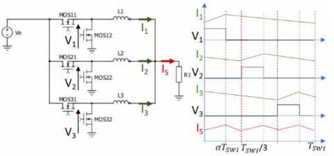
The parallel association (Multicellular buck converter) of several single-cell converters (N cells) makes it possible to reach a high power without increasing constraints on the power switches (Figure 3). The output current is distributed on cells which implies an equal repartition of losses and components heating on phases [9, 10].
In this configuration, each cell is controlled with the same duty cycle α and the same switching frequency (FSWI) (Figure 3). Interleaved control which consists of phase shift of (2π/N) of the switching orders between two adjacent cells helps to reduce the current ripple at the output by increasing the apparent output switching frequency (Figure 3) [11, 12]. In this converter, independent inductances with the same value are placed in each cell to reduce the current ripple on the phases.
Figure 3. Multicellular buck converter with independent inductances (example: 3 cells)
This topology main drawback is the high current ripple in each phase which leads to higher AC Joule losses. Unlike the output current ripple, the phase currents are not reduced, and their ripple increase with the cell number (Eq. 3) [12]. Thus, this topology is not convenient for a high number of cells.
$\frac{\Delta I_{p h}}{I_{p h}}=N^2 \frac{\Delta I}{I}$ (3)
Magnetic coupling of inductances is the solution to maintain the advantages of the multicellular converter while avoiding the strong current ripple in phases [6, 7]. The current ripple in each phase is reduced due to the increase of switching frequency on phase current. The topology is presented in the next section.
3.2 Magnetically coupled structures
Magnetic coupling increases the apparent frequency on phase currents which lead to a significantly reduced current ripple. Consequently, magnetic coupler improves converter efficiency since copper losses related to AC components are reduced. In addition to efficiency improvement, magnetic coupling offers a volume saving compared to independent inductances topology. That is why this type of converter provides a very high-power density.
Figure 4. Monolithic coupler
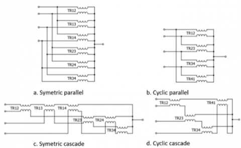
A single magnetic core [13, 14] (known as monolithic structures) (Figure 4) or several separate transformers [6, 12] (Figure 5) can be used to couple all phases. The main drawback of the monolithic structure is the complexity of building the magnetic core [15]. The use of separate intercell transformers (Figure 5) improves the coupler modularity and greatly improves its practical implementation. In fact, the magnetic coupler is made using standard commercial core shapes U, E and I. Cyclic parallel and cyclic cascade topologies are interesting (Figure 5b-d) since for a N phases converter they only require N transformers [15]. The cyclic cascade topology (Figure 5.d) is chosen for the implementation in the realized converter because of the low number of transformers required and its high filtering quality compared to cyclic parallel topology [15]. Another drawback of magnetic coupler is necessity of current closed loop control in order to obtain an equal repartition of the output current in phases. Indeed, from a practical point of view, the disparities between the active devices and between the passive devices cause an imbalance in the distribution of the output current between the phases which can lead to the saturation of the magnetic components.
Figure 5. Separate intercell transformers
4.1 Magnetic coupler sizing
Inverse coupling in each transformer allows a DC magnetic flux compensations which also helps to reduce the volume of the magnetic coupler. The coupler sizing will be based on AC magnetic flux ( $\emptyset_{A C 1}$ ) and must take into account phases number (N), input voltage (VE) and switching frequency (FSWI). To find the minimal section of the magnetic core (SF), the magnetic flux ( $\emptyset_{A C 1}$ ) must be calculated first (Eq. 4).
$S_F=\frac{\emptyset_{A C 1}}{B_{\max }}=\frac{\frac{1}{N_S} \int V_{L 1} d t}{B_{\max }}$ (4)
To establish the expression of the voltage across the windings (VL1), a system of equations relating the voltage across the windings and the voltage at the output of the switching cells can be determined using Kirchhoff’s voltage law. The magnetic core section is calculated for the maximum magnetic flux (Eq. 5), so the duty cycle is fixed at 50% [6].
$\emptyset_{1 A C}=\frac{V_E}{16 \cdot N_S \cdot F_{S W I}}$ (5)
Figure 6 shows the impact of increasing the switching frequency on the magnetic core section. Increasing the phases number allows to reduce the phase current and improve power repartition on cells. Nevertheless, using a high number of cells implies the use of large magnetic core due to the magnetic field increase (Figure 6).
4.2 Permutation mode
Magnetic flux can be reduced using the permuted mode which consists of changing phase shift Ө between each adjacent cell. The reorganization of the phase order in the control signals contributes to reduce the voltage across the windings and consequently the magnetic flux. The permuted mode can be used for a 5 cells minimum converter and applied using phase shift Ө that depends on phase number N [12]:
Figure 6. Magnetic core section for multiple phases number (VE=48 V; Ns=2 (number of turns))
For example, to apply the permuted mode in an 8 phases converter, a phase shift of 3π/4 between each adjacent cell is required (Table 2). To illustrate permuted mode advantages, we carried out simulations on multicellular buck converter with cyclic cascade using standard and permuted mode.
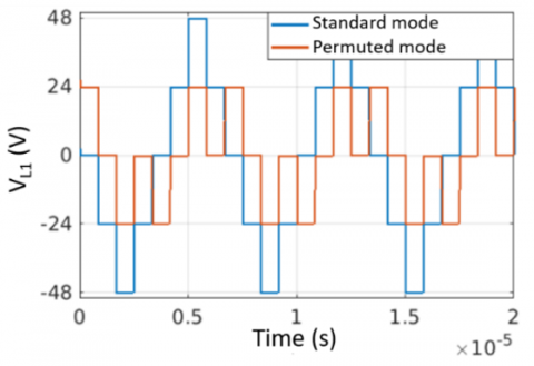
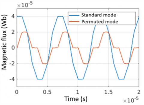
Figure 7 presents voltage across windings using standard and permuted mode for 50% duty cycle. The reorganization of phases control in this example (8 phases) implies the reduction of phase voltage from 48 V peak (input voltage) to 24 V peak. Consequently, magnetic flux is reduced by a factor of 2 (Figure 8). So, the permuted mode is an efficient method to optimise magnetic coupler volume without changing design parameters such as input voltage or switching frequency.
Figure 7. Effects of permuted mode on voltage across winding (N=8 VE=48 V α=50%)
Table 2. Permuted mode (Example N=8)
|
Phase number |
Phase shift |
Phase number |
Phase shift |
|
Phase 1 |
0 |
Phase 5 |
π |
|
Phase 2 |
3π/4 |
Phase 6 |
7π/4 |
|
Phase 3 |
3π/2 |
Phase 7 |
π/2 |
|
Phase 4 |
π/4 |
Phase 8 |
5π/4 |
4.3 Semiconductor and magnetic coupler losses
The DC/DC converter design parameters such as phase numbers, switching frequency and number of windings turns directly impact the efficiency and volume of the magnetic coupler. The semiconductors losses have 4 origins: switching losses (PSWI), RDSON Joule losses (PJ), rectifier losses (PREC_1, PREC_2) and gate losses (PGATE). Firstly, switching losses represents the wasted energy due to the state transitions and depend mainly on the switching frequency and the duration of the transient regime (Eq. 6) [12].
$P_{S W I}=\frac{1}{2} F_{S W I} V_E I_{P H}\left(t_{o n}+t_{o f f}\right)$ (6)
Figure 8. Effects of permuted mode on magnetic flux (N=8 VE=48 V α=50%)
Joule losses (PJ) on MOSFETs are proportional to drain source resistor (RDSON) and the phase current (IPH) (Eq. 7). The MOSFETs rectifier losses have two sources: dead time between MOSFETs controls (Eq. 8) and reverse recovery current (Eq. 9).
$P_I=R_{D S O N} I_{P H}^2$ (7)
$P_{R E C_{-} 1}=t_d V_F I_{P H} F_{S W I}$ (8)
$P_{R E C_{-} 2}=V_E Q_{r r} F_{S W I}$ (9)
The input capacitance Ciss of MOSFETs creates supplementary losses due to the charging and discharging cycles (Eq. 10) [12].
$P_{G A T E}=V_G Q_G F_{S W I}$ (10)
The windings of the magnetic coupler involve Joule effect losses related to the volume of copper and the current density (Eq. 11). Other sources of losses in the magnetic core are eddy currents and hysteresis cycle. Iron losses depend on the waveform of the magnetic flux, switching frequency and the magnetic core properties. PSIM® simulations on a 4 phases cyclic cascade coupler show quasi sinusoidal waveforms of the magnetic flux (Figure 8). Thus, Steinmtez model can be used to model losses in the transformer (Eq. 12). The magnetic material coefficients such as K, a and b are deduced empirically from material’s hysteresis curve using curve fitting.
$P_{\text {WIN }}=\rho J V_{\text {WIN }}$ (11)
$P_{I R O}=K F_{S W I}^a B_{\text {peak }}^b V_{T R A}$ (12)
4.4 Multicriteria optimization
To assess the impact of each design parameter, we calculated the losses in the semiconductors and the magnetic coupler considering a large range of phase numbers and switching frequencies (Figure 9). The losses are calculated considering:
The losses in the semiconductors tend to decrease when the number of phases increases as shown in Figure 9. Increasing the number of phases reduces the current in each phase, which helps to reduce the Joule effect losses. However, a high number of cells implies the use of a large number of transformers, which increases the iron losses.
Table 3. MOSFET characteristics
|
Parameter |
Value |
|
VDS |
80V |
|
ID |
300A |
|
RDS |
1.4mΩ |
|
VGS |
∓20V |
|
ton |
19ns |
|
toff |
55ns |
|
Qg |
231nC |
|
Qrr |
177nC |
Figure 9. Losses evolution on semiconductors and magnetic coupler for multiple phases number
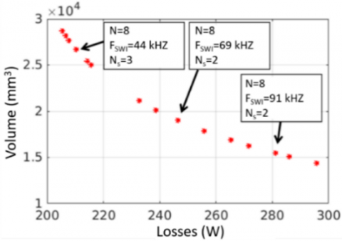
On the other hand, increasing the switching frequency is beneficial to optimize the volume of the magnetic components, but it also leads to an increase in the switching losses in the semiconductors as well as the iron losses of the magnetic coupler. It finally appears that design parameters such as phases number N, switching frequency FSWI and number of turns per winding Ns affect, in different ways, the volume of the magnetic component as well as the converter efficiency. Therefore, we decided to use NSGA-II genetic algorithm to optimize the magnetic coupler volume and the converter efficiency (Eq. 13). In order to respect some practical constraints, search space is limited (Eq. 14).
$\min \left\{\begin{array}{c}f_{\text {losses }}=P_J+P_{S W I}+P_{I R O}+P_{W I N} \\ f_{\text {volume }}=X\left(A_W \cdot A_C\right)^{\frac{3}{4}}\end{array}\right.$ (13)
$\left\{\begin{array}{c}N \in[3 ; 8] \\ N_S \in[1 ; 4] \\ F_{S W I} \in[40 ; 100] k H z\end{array}\right.$ (14)
Figure 10. Pareto front representing the optimum conception parameters for I=600 A VE=48 V
The optimization algorithm calculates the optimum design parameters taking into account input voltage, output current, MOSFETs characteristics, current density and magnetic material properties. Each point on the Pareto front (Figure 10) represents an optimum combination of phases number (N), switching frequency (FSWI) and number of turns on the windings (NS). For the studied switching frequency range [40; 100] kHz, the optimization algorithm converged to a number of 8 phases and 2 or 3 turns on windings. To simplify the practical implementation of the magnetic coupler, we choose a number of 2 turns for the windings.
4.5 Converter simulations
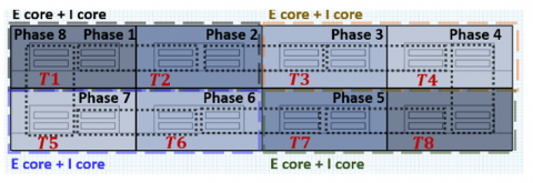
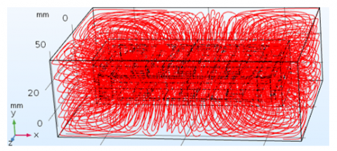
The multi-objective optimization presented in last section shows that 8 phases represent the best compromise between converter efficiency and volume of magnetic coupler. Before practical realization of the converter, we propose to verify the converter performance with the optimum conception parameters by simulations. The particularity of the chosen software (PLECS) is the possibility of coupling different circuits such as electric, magnetic and control circuits. The model takes into account the magnetic coupler dimensions and magnetic properties such as permeability and leakage inductance. The 8 phases magnetic coupler is realized using 4 magnetic cores with “E” form and 4 magnetic cores with “I” form. The assembled magnetic core is equivalent to 8 transformers (Figure 11).
Figure 11. 8 phases magnetic coupler
Given the targeted switching frequency range [40;60 kHz] and input voltage (48 V) constraint, we decided to use an E58 magnetic core that presents 150 mm² core section and leads to a 26,5 µH magnetizing inductance per transformer. The converter simulation using PLECS software requires magnetic coupler dimensions and leakage inductance values. For this purpose, COMSOL simulation software have been used in order to calculate magnetic energy in the magnetic coupler which allows us to deduce leakage inductance value (Eq. 17). 2D and 3D simulations (Figures 12-13) were compared to analytic results (Eq. 18) to validate the simulation model (Table 4). Leakage inductance obtained in 3D simulation (Figure 13) has a higher value (+46%) compared to the 2D and the analytical equation.
Table 4. Magnetic energy and leakage inductance
|
|
Analytic |
2D Sim. |
3D Sim. |
|
Emf Emc Lff Lfc |
1,2 mJ 9,8 mJ 244,05 nH 30,05 nH |
1,23 mJ 9,85 mJ 246,39 nH 30,79 nH |
1,8 mJ 14,43 mJ 360,86 nH 45,1 nH |
In 3D simulation, leakage fluxes caused by coil ends are computed and included in simulation unlike the 2D simulation (Figure 12) and analytic equation. Thus, leakage inductance obtained using 3D simulation will be used in PLECS software for converter simulation.
$L_{f f}=\frac{2 W_{m c}}{N \cdot I_{p h}^2}$ (15)
$L_{f f}=\mu_0 l_{a v} \frac{N_s}{h}\left(\frac{2 b_1}{3}+b_2\right)$ (16)
Figure 12. Leakage flux (white contours) in 2D simulation
Figure 13. Leakage flux (red contours) in 3D simulation
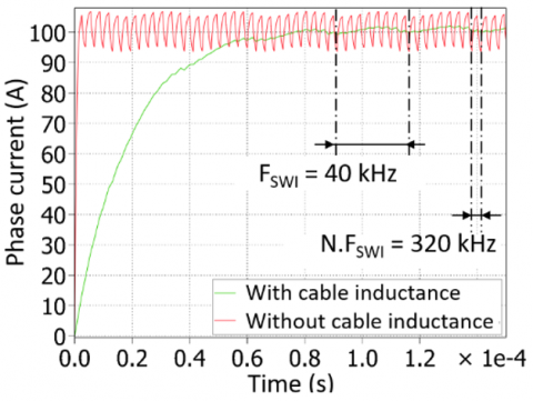
In PLECS simulation model, the control signals are connected to MOSFETs gate and each phase of the converter is connected to magnetic circuit through a magnetomotive force. In each transformer window, we placed leakage permeance to take into account effects of leakage fluxes. At the converter output, equivalent model of a 5 meters-long-cable which represents a 56 mΩ resistance in series with a 1 µH inductance is connected. In these simulations, the input voltage is fixed (VE=48 V) as well as the switching frequency (FSWI=40 kHz).
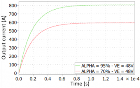
The simulations carried without taking into account the cable inductance (Figure 14) highlight the advantages of the magnetic coupler in this application. In fact, the ripple frequency of the phase currents is 8 times higher (320 kHz) than the switching frequency (40 kHz), which helps to significantly reduce the amplitude of the current ripple. This current ripple is conditioned by the leakage inductance. At the same time, the magnetizing inductance has an impact on the current ripple at the switching frequency (40 kHz). The simulations also show that the cable inductance has a significant effect on the phase current waveforms. The phase current ripple (Figure 14) is significantly reduced when the simulation takes into account the cable inductance. The output currents (Figure 15) obtained in these simulations confirm that the multi-cell inverter can significantly reduce the current ripple by increasing the apparent switching frequency at the output (N.FSWI). The simulations show that 600 A output current is reached with 70% duty cycle.
Figure 14. Phase current for 95% duty cycle
Figure 15. Output current for 70% and 95% duty cycles
5.1 Converter realization
After validating the design parameters of the converter using simulations, we developed a prototype converter for space charge measurement. The developed converter has 8 phases associated with a cascade cyclic coupler. Each winding consists of two copper coils with a cross-section of 12 mm² and a thickness of 1.5 mm. The 8 phases magnetic coupler is built using E58 magnetic cores. Closed-loop control of the converter is achieved by measuring the current in each phase using LEM HASS 100-S Hall Effect current transducers which can measure up to 100 A with an accuracy of 1 A.
Figure 16. Converter 3D overview
The eight switching cells are distributed on two identical PCBs each supporting four phases to ease the connection with the magnetic coupler (Figure 16). Another board contains a microcontroller and an FPGA connected to the MOSFET drivers. This control board is used to drive the converter to obtain the desired pulse and to adjust the duty cycles to balance the phase currents. The FPGA produces the PWM signals for the 16 MOSFETs (Table 3) in the converter, while the microcontroller sends the duty cycle settings from the controller to the FPGA using the SPI link. An additional advantage of using a microcontroller in our system is the simplification of phase currents acquisition and their associated calculations as the microcontroller includes analogue/digital converters and an FPU. This makes it easier to perform floating point calculations with the microcontroller compared to the FPGA. The microcontroller is also connected to the computer via an isolated Ethernet link.
5.2 Open-loop tests with resistive charge
Figure 17. Control signals of the phases 1 and 2 (Vgs) FSWI=43 kHz VE=5 V α=25%
Before testing at the nominal power, we performed functional tests of the converter on a resistive load (R=100 mΩ). The control signals were carefully analyzed because a precise phase shift between the control signals is necessary in order not to unbalance the magnetic coupler. A phase shift of 45° corresponding to 360° divided by 8 is imposed between the control signals of two adjacent cells (phase 1 and 2) (Figure 17). This test also makes it possible (by sending an imposed value of the duty cycle) to confirm the correct operation of the Ethernet link between the computer and the control board as well as the link between the FPGA board and the microcontroller.
5.3 Closed-loop tests with standard mode on 5 meters-long cable
The first method tested to balance the current between phases is based on the use of 8 independent PI controllers with the same reference which is equal to the output current divided by the number of phases. To improve closed-loop dynamic performance without causing instability, the coefficients of the PI controllers automatically adjusted for transient and steady state conditions. during the transient state, the integral coefficient has a higher value (Ki=1/15) in order to reduce the current rise time. As the phase current approaches the reference, the integral coefficient will be divided by 5 (Ki=1/75). The proportional coefficient is set to Kp=1/10 during these tests.
Figure 18. Phase currents for 550 A output current reference (FSWI=43 kHz VE=44 V Kp=1/10 Ki=1/15)
Figure 19. Output current for 300, 400 and 550 A output current reference (FSWI=43 kHz VE=44 V Kp=1/10 Ki=1/15)
Figure 18 shows the phase currents for output current reference of 550 A over a duration of 200 ms. The phase currents are superimposed, which validates the closed loop operation. The output currents for three different references (300, 400 and 550 A) show that the dynamics of the closed loop under these conditions is not suitable to reach the current reference in the desired time (Figure 19). The increase in the reference value of the output current is associated with an increase in the discharge rate of the power source (here a 160 F / 48 V super capacitor). Therefore, the closed loop must have a very high dynamic range in order to compensate for the drop in the voltage of the power source. Despite the adjustment of the closed loop parameters, no satisfactory combination that would significantly improve the current dynamics without degrading the stability has been found.
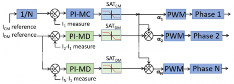
The second method that has been tested involves two different types of controllers (Figure 20) for current balancing [15]. Firstly, the common value controller (PI-MC) sets an identical output current reference for all phases (the total output current desired is divided by N, the number of phases) Secondly, the differential value controllers calculate an additional duty cycle to minimize the current difference between the reference phase and the other phases (α2 … αN) (Figure 20). Under these conditions, the output current dynamics will be mainly impacted by the characteristics of the common value controller. On the other hand, differential value controllers do not require high dynamics since they only adjust duty cycles for current balancing.
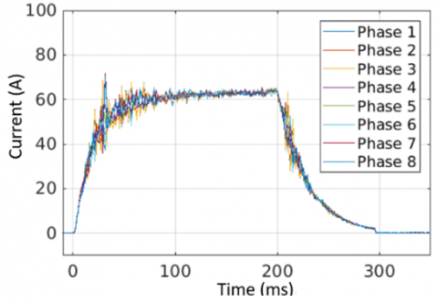
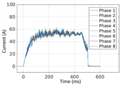
In the case of an 8-phase converter, a single common value controller is used to set the phase current and 7 differential value controllers are used to minimise the current imbalance between the reference phase and the other phases. The input reference of the common mode controller is the output current for one phase, while the differential value controllers have a current reference of 0 A. The proposed method is tested for 450 A output current reference which represents a current of 56 A in each phase (Figure 21).
Figure 20. Principle of common mode and differential mode controllers
Figure 21. Phases current for 450 A output current reference (FSWI=43 kHz VE=44 V KpCM=1/70 KiCM=1/40 SATCM=95% KpDM=1/100 KiDM=1/70 SATDM= ±5%))
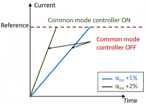
The measured phase currents in this test validate the control technique as the desired output current is achieved. The perfect superposition of the phase currents is an indication of the good performance of the differential controllers in balancing the current in the phases. The closed-loop tests (Figures 18-21) show the effect of the regulators on balancing the current in the phases of the magnetic coupler. However, the closed-loop dynamics of the converter is slower than in the open loop and makes it more difficult to generate high amplitude with short duration (≈100 ms) current pulses. To improve the current dynamics, we propose a hybrid control mode between open and closed loop. The hybrid control helps to reduce the rise time of the converter output current and still allows a current balancing during the pulse. The proposed method consists on replacing the common controller with a linear duty cycle slope (increase each 250 µs) during transient state (Figure 22). During this phase, the 7 differential controllers are still activated. In this case, the current dynamics will be impacted by the duty cycle increment step (αinc) to reach the set point in the desired time. Once the current reference is reached, common value controller is activated to maintain the output current at the set point. During the current pulse, all the 7 differential controllers are activated to force current balancing.
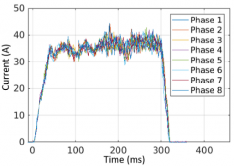
The proposed method was first tested for an output current reference of 300 A for 300 ms. The measurement of the current in the other phases confirms an equal distribution of the output current over the phases (Figure 23). In this test, the duty cycle step in the rising phase is αinc=0.3%. To check the influence of this parameter on the output current dynamics, we performed tests with different values of αinc (Figure 24). The tests show that the hybrid control is suitable for applying very short current pulses (<100 ms) in the studied cable.
Figure 22. Hybrid control to improve output current dynamics
Figure 23. Phases current for 300 A output current reference (FSWI=43 kHz VE=40 V KpCM=1/70 KiCM=1/30 SATCM=95% KpDM=1/100 KiDM=1/70 SATDM= ±5%))
Figure 24. Output current for 300 A reference (FSWI=43 kHz VE=40 V KpCM=1/70 KiCM=1/30 SATCM= 95% KpDM=1/100 KiDM=1/70 SATDM= ±5%))
5.4 Closed-loop tests with permuted mode on 5 meters-long cable
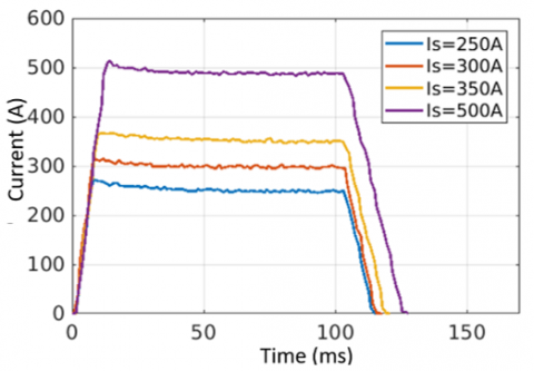
To improve the performance of the converter and especially the magnetic coupler, a permutation of the order in which the phases are controlled is applied with a switching frequency of FSWI=60 kHz. In permuted mode, the voltage across the windings is divided by 2 which reduce the magnetic flux. Increasing the switching frequency to FSWI=60 kHz combined with the permuted mode significantly reduce the magnetizing currents in the magnetic coupler, which improves the phase current waveforms (Figure 25).
Phase currents measurements validate the balancing of the output current in the phases and high current dynamics, allowing the output current reference to be reached after a few milliseconds (Figure 26).
Figure 25. Phases current for 250, 300, 350 and 500 A reference (FSWI=60 kHz VE=45 V αinc=1.4%)
Figure 26. Output current for 250, 300, 350 and 500 A reference (FSWI=60 kHz VE=45 V αinc=1.4%)
5.5 TS current measurements
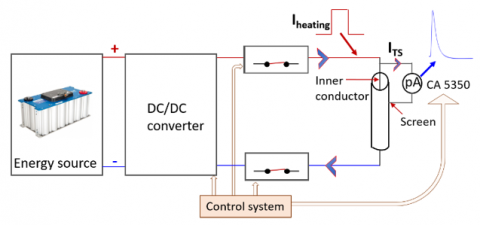
The space charge measurement bench consists of a DC power source, a DC/DC converter, a control system, two relays and a CA5350 current amplifier (Figure 27). The relays provide electrical separation between the cable and the converter during TS current measurements. The electrical separation of the cable and the converter prevents the TS current measurement from being disturbed by MOSFET leakage currents. The NI Labview control system allows the converter to be controlled to apply a current pulse, control the relays and adjust the current amplifier settings. To measure space charge, the following steps are performed by control system:
Figure 27. Space charge measuring bench overview
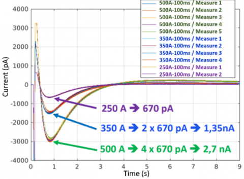
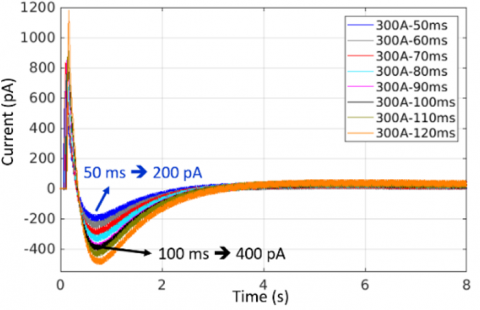
TS current measurements were performed to validate the TSM principle after electrical and thermal conditioning of the cable to be measured under 30 kV at 50°C during 44 hours. The TS measurements (Figures 28 and 29) show the proportionality between the amplitude of the power pulse applied to the cable core and the measured TS current which confirms the measurement principle. The TS current evolution is in accordance with TSM theory (Eq. 1-2) since the measured current amplitude depend on the square of heating current (Figure 28) and is proportional to heating current duration (Figure 29). The reproducibility of the measurements was also verified by performing several measurements with the same power pulses on the cable core (Figure 28).
Figure 28. TS current measurements for different power pulses amplitudes
Figure 29. TS current measurements for different power pulses durations
In this paper, a simulation and experimental study on the implementation of a “non-intrusive” space charge measurement bench in long length of insulated cables is detailed. The TSM simulations shown in the first section have enabled the estimation of the power pulse required to induce a measurable TS current. In the second section, a converter structure suitable for high current applications has been presented to generate heating current pulses on the cable conductor. First, using numerical simulations, we validated the operating principle of the converter with optimized design parameters. Next, a prototype converter was developed to provide a controlled heating current pulse in the cable core in terms of amplitude, dynamic and duration. Measurements carried out on a 5 meters-long cable confirm that the targeted heating current (500 A) is achieved with a high dynamic range that allows a short current pulse (100 ms) to be applied. The closed-loop control of the converter ensures that the heating current reference is achieved and that the currents in the phases remain balanced, preventing saturation of the magnetic coupler and helping to protect against current overloads. Finally, using the developed and designed space charge measurement bench, the principle of measurement is validated on a 5 meters long cable by performing a TS current measurement. The accordance between the applied power pulse and the amplitude of the measured TS current confirms the measurement principle.
The results obtained make it possible to estimate the distribution of the space charge present within the cable insulation. Monitoring this charge distribution makes it possible to detect areas in which the electric field may become destructive. This paper has introduced a new, flexible, light and easy to implement measurement method of space charges on long cables, contrary to the usual methods requiring the use of heavy and cumbersome means and not being able to measure on cables whose length exceeds a few dozen of centimeters. In addition, the combination of several converters in parallel makes it possible to facilitate the increase of the injected current, which makes it possible to work on cables with a large cross-section and a long length and thus avoid all the inconveniences introduced by the use of AC current to generate the power pulse.
|
AC |
Section of the magnetic core (m2) |
|
AW |
Windings surface (m2) |
|
b1 |
Coil width (m) |
|
b2 |
Distance between coils in window area (m) |
|
Bmax |
Maximum magnetic flux density supported by magnetic material (T) |
|
Bpeak |
Magnetic flux density (T) |
|
C |
Cable capacitance (C) |
|
Cp |
Heat capacity of the conductor (J. Kg-1. K-1) |
|
E |
Electric field (V/m) |
|
FSWI |
Switching frequency (Hz) |
|
flosses |
Converter losses (W) |
|
fvolume |
Magnetic coupler volume (m3) |
|
h |
Height of window area (m) |
|
I |
Output current (A) |
|
Iph |
Phase current (A) |
|
ITS |
Thermal step current (A) |
|
J |
Phase current density (A.m-2) |
|
K, a, b |
Magnetic material coefficients given in datasheet |
|
Ki |
Integral coefficient of PI controller |
|
Kp |
Proportional coefficient of PI controller |
|
lav |
Average length of coil (m) |
|
Lfc |
Leakage inductance in coupler (H) |
|
Lff |
Leakage inductance in transformer (H) |
|
m |
Conductor weight (Kg) |
|
PIRO |
Iron losses of magnetic coupler (W) |
|
PJ |
Joule losses on MOSFETs (W) |
|
PREC1 |
Dead time diode losses (W) |
|
PREC2 |
Reverse recovery losses (W) |
|
PSWI |
Switching losses (W) |
|
PWIN |
Joule losses on windings (W) |
|
QG |
Gate charge (C) |
|
Qrr |
Reverse recovery charge (C) |
|
R |
Conductor resistance (Ω) |
|
RDSON |
Drain-Source on resistance (Ω) |
|
Re |
Outer radius of insulation (m) |
|
Ri |
Inner radius of insulation (m) |
|
SAT |
Output saturation of PI controller (%) |
|
SF |
Section of the magnetic core (m2) |
|
td |
Dead time between MOSFETs control of the same cell (s) |
|
toff |
Turn-off delay time (s) |
|
ton |
Turn-on delay time (s) |
|
tpulse |
Current pulse duration (s) |
|
VE |
Input voltage (V) |
|
VF |
Diode forward voltage drop (V) |
|
VG |
Gate voltage (V) |
|
VL1 |
Voltage across the winding (V) |
|
VTRA |
Transformer volume (m3) |
|
VWIN |
Copper volume of windings (m2) |
|
Wmc |
Magnetic energy in coupler (J) |
|
Wmf |
Magnetic energy in transformer (J) |
|
X |
Geometric coefficient of (E+I) core shape |
|
Greek symbols |
|
|
$\alpha$ |
Coefficient of the capacitance variation with temperature (K-1) |
|
∆T |
Temperature variation (K) |
|
$\emptyset_{1 A C}$ |
Magnetic flux (Wb) |
|
Ɵ |
Phase shift between two adjacent cells (rad) |
|
$\rho$ |
Copper resistivity (Ω.m) |
|
µ0 |
Vacuum magnetic permeability (H.m-1) |
|
Subscripts |
|
|
CM |
Common mode |
|
DM |
Differential mode |
|
TS |
Thermal step |
[1] Castellon, J., Agnel, S., Toureille, A., Brame, F., Mirebeau, P., Matallana, J. (2009). Electric field and space charge measurements in thick power cable isulation. IEEE Electrical Insulation Magazine, 25(3): 30-42. https://doi.org/10.1109/MEI.2009.4977240
[2] Hascoat, A., Castellon, J., Agnel, S., Frelin, W., Egrot, P., Hondaa, P., Le Roux, D. (2014). Study and analysis of conduction mechanisms and space charge accumulation phenomena under high applied DC electric field in XLPE for HVDC cable application. In 2014 IEEE Conference on Electrical Insulation and Dielectric Phenomena (CEIDP), Des Moines, IA, USA, pp. 530-533. https://doi.org/10.1109/CEIDP.2014.6995877
[3] Agnel, S., Notingher, P., Toureille, A. (2000). Space charge measurements under applied DC field by the thermal step method. Annual Report Conference on Electrical Insulation and Dielectric Phenomena, Victoria, Canada, pp 532-535. https://doi.org/10.1109/CEIDP.2000.885253
[4] Castellon, J., Agnel, S., Toureille, A., Frechette, M. (2008). Space charge characterization of multi-stressed microcomposite nano-filled epoxy for electrotechnical applications. Annual Report Conference on Electrical Insulation and Dielectric Phenomena, Quebec, Canada, pp 166-170. https://doi.org/10.1109/CEIDP.2008.4772875
[5] Agnel, S., Notingher, P., Toureille, A., Castellon, J., Malrieu, S. (1999). Study of space charge dynamics directly on power cables using the thermal step method. Annual Report Conference on Electrical Insulation and Dielectric Phenomena, Austin, USA, pp 50-53. https://doi.org/10.1109/CEIDP.1999.804590
[6] Darkawi, A., Martire, T., Notingher, P., Huselstein, J.J., Forest, F., Enrici, P. (2013). A high current multi-cell buck converter using intercell transformers: Modeling and design of a 1200 amps, 12-phase prototype. In 2013 15th European Conference on Power Electronics and Applications (EPE), Lille, France, 1-9. https://doi.org/10.1109/EPE.2013.6631915
[7] Darkawi, A., Martire, T., Huselstein, J.J., Forest, F., Notingher, P. (2013). Modeling and design of multi-cell buck converters using InterCell Transformers for HVDC cable diagnostic. In 2012 38th Annual Conference on Industrial Electronics Society (IECON), Montréal, Canada, 561-566. https://doi.org/10.1109/IECON.2012.6388670
[8] Castellon, J., Agnel, S., Notingher, P. (2017). Review of space charge measurements in high voltage DC extruded cables by the thermal step method. IEEE Electrical Insulation Magazine, 33(4): 34-41. https://doi.org/10.1109/MEI.2017.7956631
[9] Hayashi, Y., Matsugaki, Y., Ninomiya, T., Kose, S., Tanoue, H. (2017). Transformerless multicellular dc-dc converter for highly efficient next generation dc distribution system. IEEE International Conference on Power Electronics, Drives and Energy Systems (PEDES), Warsaw, Poland, pp 1-9. https://doi.org/10.23919/EPE17ECCEEurope.2017.8099166
[10] Garg, A., Das, M. (2021). High efficiency three phase interleaved buck converter for fast charging of EV. 1st International Conference on Power Electronics and Energy (ICPEE), Bhubaneswar, India, pp 1-5. https://doi.org/10.1109/ICPEE50452.2021.9358486
[11] Cougo, B. (2010). Design and optimization of intercell transformers for parallel multicell converters (Doctoral dissertation, Institut National Polytechnique de Toulouse-INPT).
[12] Bouhalli, N. (2009). Etude et intégration de convertisseurs multicellulaires parallèles entrelacés et magnétiquement couplés (Doctoral dissertation). INP Toulouse.
[13] Forest, F., Meynard, T.A., Laboure, E., Costan, V., Sarraute, E., Cuniere, A., Martire, T. (2007). Optimization of the supply voltage system in interleaved converters using intercell transformers. IEEE Transactions on Power Electronics, 22(3): 934-942. https://doi.org/10.1109/TPEL.2007.897089
[14] Meynard, T., Forest, F., Laboure, E., Costan, V., Cuniere, A., Sarraute, E. (2006). Monolithic magnetic couplers for interleaved converters with a high number of cells. In 4th International Conference on Integrated Power Systems, 1-6. VDE. Naples, Italy
[15] Sanchez, S. (2015). Contribution à la conception de coupleurs magnétiques robustes pour convertisseurs multicellulaires parallèles (Doctoral dissertation).