Fatima Zohra Boukahil* | Omar Charrouf | Sabrina Abdeddaim | Achour Betka | Abdelkrim Menadi
© 2022 IIETA. This article is published by IIETA and is licensed under the CC BY 4.0 license (http://creativecommons.org/licenses/by/4.0/).
OPEN ACCESS
This paper investigates the performances analysis of PV-RO desalination system under uniform and non-uniform irradiance conditions. The main objective is the application of Extremum Seeking Control (ESC) to the GPV side in order to overcome the generated power and water quantity losses to improve the performance of the whole system. The technical design of the developed system is based on an existing RO desalination unit beside that real climatic data taken from a local mast are involved in this study. The modeling of the whole system and the control techniques adopted in this study are fully formulated. The whole system is modeled and controlled using MATLAB/Simulink. Different scenarios (healthy and shaded) based on real climatic data have been used to carry out the results. The ESC used shows its effectiveness to extract maximum power under shaded conditions for all the proposed scenarios. Compared with conventional controllers, this technique can offer extra power surrounding 685W in several cases. Furthermore, the shading conditions can affect widely freshwater production whose losses are estimated at around 82.91% for critical scenarios. The findings results are very significant for industrialists working in this field.
desalination, extremum seeking control (ESC), MATLAB/Simulink, maximum power point tracking (MPPT), perturb and observe (PO), photovoltaic (PV), reverse osmosis (RO), shading
The international community is facing a serious challenge to assume the growing demand for fresh water in many regions of the globe. Indeed, technological and social development urges scientific researchers to diversify the freshwater resources in order to fit with the population growth. Although the abundance of water on the earth is about 97% salty, freshwater represents only 3% of the total resources [1]. Today, due to industrial development, agricultural intensification, improvement of living conditions, and massive population growth, there is a rising demand for freshwater [2, 3]. In order to cope with this predicted water shortage, converting seawater or brackish water into drinking water to ensure enough of the current demand for freshwater, desalination technology is seen as a promising solution [4]. Most of these desalination systems are located in arid climate regions which can be desert or semi-desert, disposing of an important solar and wind energy potential, such as Algeria or North Africa [5]. In the areas where the grid is generally not available, this technology is considered an avoidable technical orientation due to the large amount of energy required for the desalination process. The cost per cubic meter (m3) of desalinated water is relatively high in remote areas nevertheless connected to the power grid can be more expensive [6]. Among the renewable energy sources, the use of solar energy is considered the best solution for desalination technology, especially in remote and arid regions [7].
Two main desalination processes achieving technological maturity are thermal-based and membrane-based. The first one acts on the basis of a phase change (liquid-vapor), while the second process is based essentially on filtration membranes. Thermal-based technologies operate on the basis of supplying thermal energy to seawater to evaporate water and then condense this vapor to obtain potable water. Thermal technologies tend to be used in regions where water salinity levels are high and energy costs are low, such as in the Caribbean and the Middle East [8]. Its main advantage is the absence of the fouling problem occurring in the membrane technology. Some examples of the most common thermal-based processes are multi-stage flash (MSF), multi-effect distillation (MED), and vapor compression distillation [9]. Although thermal technology has been widely used, membrane-based technology has become more and more popular within the geographical region like the Middle East due to its lower specific energy consumption, lower environmental footprint, and more flexible production capacity [10]. Some membrane technologies include ultrafiltration, electro-dialysis, and reverse osmosis [11]. Reverse osmosis (RO) is now the foremost commonly used desalination process worldwide, comprising 61% of the global share, followed by MSF at 26% and MED at 8% [12]. RO is capable of treating a vast range of solute concentrations in water at a reasonable cost compared to other techniques. It can also provide higher water recovery rates than multi-effect and multi-stage flash distillation. In addition, RO has lower emissions than thermal-based desalination methods. Reverse osmosis is based on the application of excessive pressure to reverse the spontaneous osmosis process, where water in solution moves across a semi-permeable membrane from lower to higher solute concentration. In reverse osmosis plants, this overpressure is applied by high-pressure pumps in order to push seawater and brackish water through semi-permeable membranes to obtain desalinated water [13].
Many countries are using desalinated water in agriculture with different ratios. Spain is the country with the highest proportion of desalinated water used for agriculture, with a current installed capacity of 1.4 million cubic meters per day, 22% of this amount is used for agriculture of high-value crops, such as vegetables, fruits (including tomatoes and peppers), and Vineyard with grapes. In Kuwait, the current installed capacity exceeds 1 million cubic meters per day whom 13% is used for agriculture; Saudi Arabia is the world's largest single producer of desalinated water; only 0.5% of its desalination capacity is employed for agricultural purposes. Other countries using desalinated water for food production are Italy (with a desalination capacity of 64,700 cubic meters/day whom 1.5% dedicated to agriculture), Bahrain (620,000 cubic meters/day, with the ratio of 0.4% for the agriculture ) while in Qatar and the United States are respectively 0.1% and 1.3% [14].
Solar thermal and photovoltaic are the two main categories involved in the desalination industry [15]. Generally, the photovoltaic source is associated to controlled converters whose purpose is tacking the maximum power point (MPP) of the P-V curve to ensure better energetic yield of the system. For a PV array, under uniform irradiance condition (UIC), MPP tracking (MPPT) algorithms such as Hill climbing (HC), Perturb and observation (P&O), and Incremental conductance (IC) can effectively achieve their goal [16] due to their simplicity of implementation. In industry, several application systems, using as a prime source a photovoltaic array, either in on-grid or off-grid, are used worldwide, where the optimization of the extracted PV power has to be tracked. The concept of these conventional methods is in fact similar. It is based on perturbing the system voltage/duty cycle and checking the evolution of the extracted power, and consequently, leads to an improvement of the overall system efficiency. However, under partially shaded conditions (PSC) these methods present certain insufficiency. In PSCs, PV modules do not receive equal solar irradiance, and the array P-V characteristic may contain a maximum peak named GMPPT (Global Maximum Power Point) and one or multiple peaks with different power values seen as LMPPT (Local Maximum Power Point) [17]. In most cases, PSCs are inevitable, especially in PV systems installed in urban areas or places with significant cloud cover. Therefore, PSC analysis and mitigation effects studies have been conducted offering the appropriate technical solutions. Accordingly, numerous MPP tracking methods for PV systems under PSC have been tested [18]. As mentioned, in the case of partial shading phenomena, more than one optimum point is remarked, located at the knees of the P-V characteristic. Among these points, only the so-called ‘global optimum point’ permits to get higher power quantities. To perform an effective tracking of this point, Meta-heuristic optimization methods can generally called. These techniques are various and have the same concept of search. Genetic Algorithm [19], Particle Swarm [20], Grey wolf [21], and others, allow through a random search to avoid stagnating on the local optimum point. The ESC is one of the proposed methods, which have been considered in this study.
The integration of renewable resources in desalination has been widely discussed as an innovative approach of desalinating water in a cost-effective and environmentally friendly way [22]. Nowadays, the reverse osmosis (RO) method dominates globally as it requires only electrical energy. This process is known to be the most appropriate and the least expensive process for seawater desalination because of recent technological developments and lower energy requirements compared to thermal processes. Furthermore, the RO process can operate with renewable energy sources (RES) such as photovoltaic (PV) and wind turbines. In fact, the desalination systems by reverse osmosis represent 62% of the total RES/desalination systems installed in the world. Many simulation studies of desalination devices used with RES have been conducted. Independent reverse osmosis desalination units powered by photovoltaic and/or wind turbines and sustained by batteries have been the research theme of several works [23, 24].
In this context, this research study concerns Biskra region which is located in the southeast of Algeria (34° 48’ N and 5° 44’ E) [25]. It is one of the most suitable locations to host the first pilot projects of photovoltaic desalination plants. It is a part of the vast Algerian desert with hot and dry climate during the long summer months, and it is also progressively hotter and drier as you proceed towards the south. The sky in the desert is usually clear, which leads to a wide temperature range between night and day. In the northern part of the desert, the average maximum temperature in July and August is around 40°C as well as in Biskra. These geographical and climatic criteria favour the use of renewable energies, especially photovoltaic solar energy.
This paper is arranged as follows: Following the introduction, Section 2 presents data and materials description (Capricorn FLX Weather Stations™, Reverse Osmosis unit RO) involved in this study. In Section 3, the controller based ESC-MPPT method is explained as technique to overcome the shading cases that occurs during the day. In the last section, the results of the simulation are done using real data specific to Biskra region in the Algerian Sahara. Finally, the paper is ended by a conclusion.
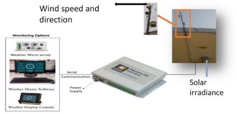
The weather data used in this study has been collected from the Capricorn FLX station located in the renewable energy laboratory in Biskra University. Figure 1 represents the weather station diagram used, which is based on many sensors such as Mechanical Wind Direction and Speed, Relative Humidity, Barometric Pressure (inside the Control Module) and Solar Irradiance.
Figure 1. System diagram of Capricorn FLX Weather station
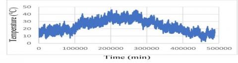
This station is used for spot measurements of temperature and irradiance, which are carried out in a similar way in the station. These measurements are taken every minute throughout the year. Figure 2 shows the profiles of solar irradiance and ambient temperature in minutes (525 600 min), over the year 2020. These profiles offer an important opportunity to study seasonal and long-term climate variations in this part of Algeria.
(a) Solar irradiance
(b) Ambient temperature
Figure 2. Meteorological parameters for Biskra over a year (2020)
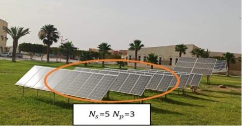
2.1 PV module field
The existing photovoltaic field in the Renewable Energy Laboratory in Biskra shown in Figure 3. is composed of 40 modules. The electrical parameters of each module are given in Table 1. For powering requirements of the existing RO unit, one used a photovoltaic generator of 15 modules (5 modules in series and 3 strings in parallel) giving an output power of 2625 W STC. The technical data of the obtained PV generator are used for the modeling and the simulation of the PV-RO system.
Figure 3. The photovoltaic field
Table 1. PV module paremeter
|
Type |
Monocristallin (Sharp) NTR5E3E/NT175E1 |
|
Maximum power |
Pmax=175.0 W |
|
Optimum current |
Iop=4.95 A |
|
Optimum voltage |
Vop=35.4 V |
|
Open circuit voltage |
Voc=44 V |
|
Open circuit current |
Icc=5 A |
|
Number of cell per module |
Ns=72 |
2.2 Installation description
The proposed battery-less PV-RO system in this preliminary design is illustrated in Figure 4. The PV generator (2340 W) is associated with an Induction Motor (IM) of 2.2 kW via a boost converter, linked to a voltage source inverter. The electrical power of the IM is converted to mechanical power to drive a high-pressure pump of 2.2 kW; which is used to transport brackish water to the RO unit by converting the kinetic energy to the hydrodynamic power of the water flow. The feed water passes throw the RO membrane under a high pressure to overcome the osmotic one. At the outlet of the RO membrane, two outputs are distinguished: brine with high concentrate salt and fresh water.
Figure 4. Schematic diagram showing the main components of a PV-RO desalination system
2.3 Mathematic model
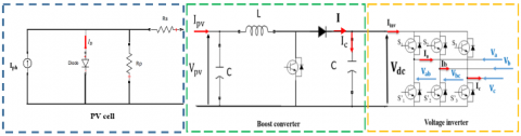
Generally, the simple PV model is based on one diode equivalent circuit shown in Figure 5 [26]. It consists of a photovoltaic current source Iph representing the irradiance, a diode representing the diffusion effect and a shunt resistor Rp, emulating losses around the junction due to impurities. A second resistor Rs connected in series emulates the joules losses.
Figure 5. Voltage source inverter connected to PV cell through a boost converter
The I-V characteristic is described by an implicit nonlinear equation:
$\mathrm{I}_{\mathrm{pv}}=\mathrm{I}_{\mathrm{ph}}-\mathrm{I}_0\left[\exp \left(\frac{\mathrm{V}_{\mathrm{pv}}+\mathrm{I}_{\mathrm{pv}} \mathrm{R}_{\mathrm{s}}}{\mathrm{a}}\right)-1\right]-\frac{\mathrm{V}_{\mathrm{pv}}+\mathrm{I}_{\mathrm{pv}} \mathrm{R}_{\mathrm{s}}}{\mathrm{Rp}}$ (1)
where,
$a=\frac{n_s \cdot A \cdot k \cdot T_C}{q}$ (2)
The energy conversion from DC to AC form is based on the combination of boost converter, which tracks the maximum power and voltage source inverter that drives the moto-pump shown in Figure 5.
The boost converter is used as an adapter impedance between the source and the load. Eq. (3) deduces the average state space model of a boost converter [27]:
$\left[\begin{array}{c}\mathrm{I} \cdot{ }_{\mathrm{pv}} \\ \mathrm{V \cdot}_{\mathrm{dc}}\end{array}\right]=\left[\begin{array}{cc}0 & -\frac{1-\alpha}{\mathrm{L}} \\ -\frac{1-\alpha}{\mathrm{C}} & -\frac{1}{\mathrm{RC}}\end{array}\right]\left[\begin{array}{c}\mathrm{I}_{\mathrm{pv}} \\ \mathrm{V}_{\mathrm{dc}}\end{array}\right]+\left[\begin{array}{c}\frac{1}{\mathrm{~L}} \\ 0\end{array}\right] \mathrm{V}_{\mathrm{PV}}$ (3)
The three-phase inverter consists of three switching arms, each one is composed of two cells with a diode and a transistor in antiparallel with DC voltage as input and three AC voltage as output [28]. The inverter is modeled by associating to each arm a logic function F that determines its conduction states: $F_i= \begin{cases}1 & \text { if } S_i \text { passing and } S_i^{\prime} \text { open. } \\ 0 & \text { if } S_i^{\prime} \text { passing and } S_i \text { open. }\end{cases}$ where i=1, 2, 3.
The following matrix equation is used to model the two-level voltage inverter:
$\left[\begin{array}{l}\mathrm{V}_{\mathrm{a}} \\ \mathrm{V}_{\mathrm{b}} \\ \mathrm{V}_c\end{array}\right]=\frac{\mathrm{V}_{\mathrm{dc}}}{3}\left[\begin{array}{ccc}2 & -1 & -1 \\ -1 & 2 & -1 \\ -1 & -1 & 2\end{array}\right]\left[\begin{array}{l}\mathrm{F}_1 \\ \mathrm{~F}_2 \\ \mathrm{~F}_3\end{array}\right]$ (4)
Eq. (5) represents the relationship between the inverter input current and the three-phase output currents:
$\mathrm{I}_{\mathrm{inv}}=\mathrm{F}_1 \mathrm{I}_{\mathrm{a}}+\mathrm{F}_2 \mathrm{I}_{\mathrm{b}}+\mathrm{F}_3 \mathrm{I}_{\mathrm{c}}$ (5)
In this article, the EBARA EVM2 22F/2.2 high-pressure centrifugal pump [29] associated with an induction motor is used. This kind of pump is widely used in moderate power applications. Three quantities, which are the flow rate Q, the pressure P and the torque Tr characterize it. The flow pressure is determined by Eq. (6):
$P=a \Omega^2+b \Omega Q+c Q^2$ (6)
The torque of the centrifugal pump, which represents the IM (Induction machine) resistant torque, is given by:
$\mathrm{T}_{\mathrm{r}}=\mathrm{a} \mathrm{Q}^2+\mathrm{b} Q \Omega$ (7)
Table 2 shows the parameters of the High Pressure (HP) pump identified from practical tests [30]:
Table 2. HP pump paremeters
|
Type |
EBARA EVM2 22F/2.2 |
|
Rated power |
2200 W |
|
Rated current |
8.71 A |
|
Rated voltage |
230 V |
|
a |
0.0002317 |
|
b |
-0.0005198 |
|
c |
-0.002427 |
In the literature, many models describe the behaviour of the membrane during its operation. It is a semi-permeable device, which separates the liquid under the pressure gradient. The RO process model is taken from the study [31], where the permeate flow rate Qp is function of Sm (the active surface of the membrane in m2), A (the water permeability Coefficient), Pf (flow pressure), and defined by the following equation:
$Q_p=A \cdot\left[P_f-\Delta \pi\right] \cdot S_m$ (8)
The behaviour of the osmotic pressure is given by:
$\Delta \pi=\mathrm{K}_{\text {nacl }}\left(T_{\text {nacl }}+273\right) \frac{C_{\text {nacl }}}{1000-\frac{C_{\text {nacl }}}{1000}}$ (9)
An important factor in the reverse osmosis process is the membrane recovery rate, which is the ratio of the flow of water produced to the feed water flow rate defined by:
$\mathrm{R}=\frac{Q_p}{Q_f}$ (10)
The efficient operation of the reverse osmosis desalination system requires applying a robust control strategy at the motor-pump side and power optimization on the PV generator side. For this reason, the Extremum Seeking Control (ESC) algorithm is used to control the boost converter linked to the PV generator, which has proven its ability to overcome the drawbacks of local-based optimization methods, to track the maximum available power in case of partial shading. On the motor side, the famous vector control is applied to convert the extracted PV power to mechanical energy at the motor shaft then to hydraulic power at the level of the RO unit.
3.1 PV generator control
Some of the traditional MPPT methods fail to track the GMPPT and cause power loses. These methods, identified as local MPPT tracking techniques present significant drawbacks in case of the partial shading state, and as consequence, have a significant effect on the desalinated water quantities. The proposed method not only focuses on the unknown nonlinear system but it is able to track the MPPT point either in healthy or in shaded cases, as shown in Figure 8.
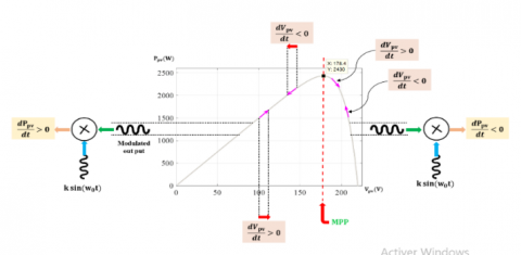
Figure 6 represents the sinusoidal ESC principal applied to the PV source. Given a nonlinear input-output map, if a sinusoidal signal of little amplitude is added to the input signal Vpv, the output signal Ppv, oscillates around its mean value. It can be observed that, when the signal Ppv, is multiplied by a sinusoidal of the same frequency and phase, the multiplier output $\frac{\mathrm{d} \mathrm{P}_{\mathrm{pv}}}{\mathrm{dt}}$ is positive before the MPP and negative at the right side of the MPP.
Figure 6. Sinusoidal ESC principal applied to PV generator
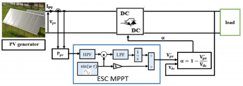
The approach can be applied to the PV system by the schema of Figure 7. The schema consists of the nonlinear Ppv, an integrator, two filters (High Pass Filter HPF and Low Pass Filter LPF) and a small sinusoidal signal. This signal is added to the PV power with the same frequency of the dither signal that is extracted through a High Pass Filter (Eq. (11)). The gradient function is the modulation by adding a sinusoidal perturbation signal (sin(ωt)) with a relatively high frequency. Then, the low-pass filter (Eq. (12)) eliminated unnecessary components and the resulting signal represented the estimated gradient [32]. The LPF output is applied to an integrator and added to k*(sin(ωt) to obtain the reference PV voltage $V_{\mathrm{pv}}^*$.
$\mathrm{HPF}=\frac{\mathrm{s}}{s+\omega_h}$ (11)
$L P F=\frac{\omega_1}{s+\omega_1}$ (12)
To ensure the convergence of the ESC controller, the cut-off frequency $\omega_h$ must be lower than the frequency $\omega_1$, and these two frequencies are much smaller than w [32].
Figure 7. Scheme of the ESC based MPPT
The main steps of the ESC based algorithm can be summarized as follows:
Step1: The injection of a small perturbation signal called the dither signal ($\operatorname{ksin} \omega t$) with a relatively high frequency to an estimate of the optimal input (Vpv*).
Step2: The PV power will have a sinusoidal component with the same frequency of the dither signal that is extracted through a High Pass Filter (HPF).
Due to the nature of the PV characteristics, this sinusoidal component is either in phase with the dither signal if the voltage is less than the MPP or out of phase if the voltage is larger than the MPP.
Step3: Multiplying the resulting sinusoid with the dither signal yields a shifted sinusoid with a positive or negative DC component if the multiplied signals are in phase or out of phase, respectively.
Step4: This DC component that is extracted through a Low Pass Filter (LPF) represents a signal proportional to the gradient of the PV power.
Step5: It is integrated and multiplied by a gradient update gain, such that the voltage estimate asymptotically approaches the MPP.
This section includes the simulation results, which have been conducted in two steps: Firstly, considering the part post DC link as fixed load seen by the DC-DC converter, the ESC control strategy is tested for two scenarios. The first one is the healthy case (without shading) for which the PV generator was tested under different irradiances and the characteristics was taken. Afterwards, the generator was simulated for another scenario (shaded case) were the GPV was made under two different irradiances. This scenario aims to see the solar irradiance fluency on the power and water quantities losses. In the last step, real data corresponding to typical dates during the year are taken as inputs and applied to the whole PV-RO system.
4.1 Healthy case
This test is designed to determine the PV generator characteristic and the maximum power generated under different irradiances in the healthy case. The results of optimum power, voltage, and current of the PV generator are given in Table 3 where the irradiance has been varied in the range 300 to 1000 W/m2. The measured power is ranging between 2430 W and 645.1W, while the voltage and the current are ranging between 187.4V-159.4V and 13.62A-4.05A respectively.
4.2 Simulation of shaded configuration
During the partial shading, the GPV receives different levels of irradiance on its area, which leads to a significant reduction of the output power. To handle that issue, for the same configuration, the GPV modules are exposed to different irradiances.
By applying the two control techniques of Maximum Power Point Tracking (MPPT): Perturb and Observe (P&O) and Extremum Seeking Control (ESC), it is found that The ESC is more valuable than P&O showing its ability to converge under the variable irradiance and converges to the GMPP while the P&O controller converges to LMPP as reported in Figure 8.
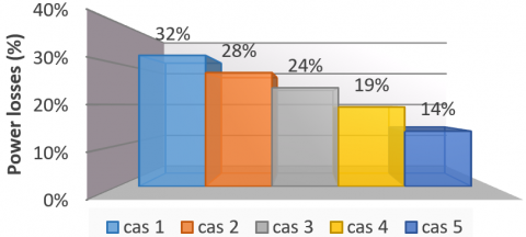
The numerical simulation results depicted in Table 4 are obtained by applying a fixed irradiance of 1000 W/m2 on eight modules while this value is changed for the rest of the field from 800W/m2 to 400W/m2 corresponding to five cases. For each one, the voltage, the current, and the power are measured. These results show that the global optimum power is ranging between 2135 W and 1441 W, while the local optimum power is ranging between 1450 W and 1246 W. The power losses corresponding to the difference between the global and the local MPPs are given in terms of percentages. It is found that the power losses for the first case achieve 32% and rise to 13.5% for the fifth case when the irradiance of the shaded part takes the value of 400 W/m2. On the other side, the water quantity ranges between 24.7% and 10.3%.
Figure 8. P-V characteristics of the shaded case
Table 3. Healthy case with different irradiances
|
E(W/m2) |
1000 |
900 |
800 |
700 |
600 |
500 |
400 |
300 |
|
Pop(W) |
2430 |
2165 |
1903 |
1644 |
1387 |
1135 |
887 |
645.1 |
|
Vop(V) |
178.4 |
177.6 |
175.2 |
172.3 |
171.1 |
167.7 |
163.9 |
159.4 |
|
Iop(A) |
13.62 |
12.19 |
10.86 |
9.54 |
8.10 |
6.77 |
5.41 |
4.05 |
Table 4. Shading effect on PV generator
|
E1 |
1000 W/m2 |
|||||||||
|
E2 |
800 W/m2 |
700 W/m2 |
600 W/m2 |
500 W/m2 |
400 W/m2 |
|||||
|
Case |
1 |
2 |
3 |
4 |
5 |
|||||
|
|
PO (local) |
ESC (global) |
PO (local) |
ESC (global) |
PO (local) |
ESC (global) |
PO (local) |
ESC (global) |
PO (local) |
ESC (global) |
|
Pop (W) |
1450 |
2135 |
1418 |
1965 |
1360 |
1792 |
1303 |
1616 |
1246 |
1441 |
|
Vop (V) |
110 |
179.2 |
115 |
179.1 |
114.3 |
178.3 |
114.4 |
178.2 |
114.1 |
176.8 |
|
Iop (A) |
13.18 |
11.92 |
12.32 |
10.97 |
11.9 |
10.05 |
11.39 |
9.07 |
10.91 |
8.15 |
|
PWQ (m3) |
1.9755 |
2.625 |
1.9611 |
2.48 |
1.9 |
2.3228 |
1.84 |
2.1565 |
1.777 |
1.982 |
|
Power Losses (%) |
32 |
27.8 |
24.1 |
19.4 |
13.5 |
|||||
|
WQL (%) |
24.7 |
20.9 |
18.2 |
14.7 |
10.3 |
|||||
|
Pop (W) (SMC) |
2035 |
1945 |
1350 |
1085 |
1245 |
|||||
|
Power Losses (%) |
4.68 |
1.02 |
24.66 |
32.86 |
13.6 |
|||||
As remarked, the first order sliding mode controller provides more much power in the two studied scenarios, but failed to track the global optimum point, and stagnate on the local optimum one in the three other situations.
Figures 9 and 10 represent the percentage of power and water quantity losses for the proposed shaded case. The following relation calculates these percentages:
Power $\operatorname{losses}(\%)=\frac{\left[P_{o p}(\text { global })-P_{o p}(\text { local })\right] \times 100}{P_{o p}(\text { global })}$ (13)
$\mathrm{WQL}(\%)=\frac{[P W Q(\text { global })-P W Q(\text { local })] \times 100}{P W Q(\text { global })}$ (14)
Figure 9. Power losses for the shaded case
Figure 10. Water quantity losses for the shaded case
The degradation of 100 W/m2 of irradiation from one case to another causes about 4.6% of power losses between the two successive cases, where it causes water quantity losses of 3.6%.
4.3 Simulation of real shading configuration
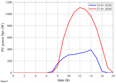
Another test was done by MATLAB/Simulink to study the influence of real data irradiance on the permeate water quantity. The simulation is carried out for 16 hours with a sampling rate of 1e-5 s. In this part, two days of January, which are 25/01/2020 and 27/01/2020 have been taken, in order to determine the quantity of water obtained.
Eq. (15) is defined to estimate the water quantity losses for the shaded day using the results obtained in Figure 10.
$\mathrm{WQL}=\frac{\mathrm{PWQ}-\mathrm{WQS}}{\mathrm{PWQ}} \times 100$ (15)
where,
PWQ is the permeate water quantity obtained by integration of the non-shaded curve of the permeate flow rate according to the following equation:
$P W Q=\int_{S R}^{S S} Q_p \mathrm{dt}$ (16)
WQS is the water quantity obtained from the shaded curve using the equation above.
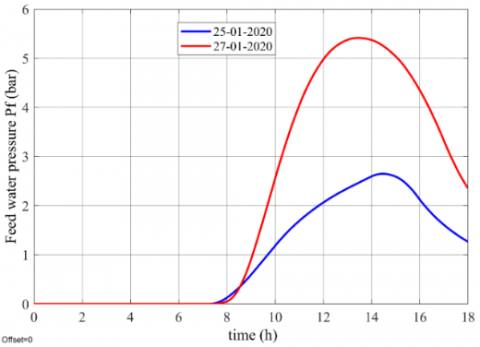
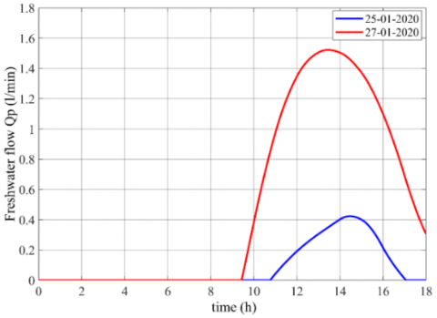
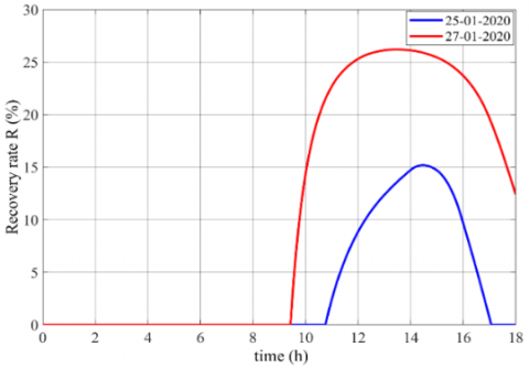
Figure 11 is represented the hourly irradiance (a), the energy delivered by the GPV (b), and the hourly hydraulic quantities: feed water pressure (c), feedwater flow (d), freshwater flow (e), and recovery (f). By analyzing the results at the true solar noon, the irradiance level is around 600 W/m2 during the healthy day, and consequently, the generated PV power is 1100 W while during the shaded day it drops under 300 W/m2 generating a PV power under 400 W. Hence, the water quantity loss is about 82.91%, corresponding to a severe shading of 50%. The hydraulic performances of the RO unit for these two days show that the feed water pressure can reach upper than 5 bar for the sunny day and do not attend 3 bar for the cloudy day. The feedwater flow is stagnating at the peak of 6 l/min for one day and is a rounding of 3 l/min for the other day.
Table 5 shows the water quantities and losses for the real scenario. It has been processed by using Eq. (15).
The Feed Water Quantity (FWQ) is calculated as follows:
$\mathrm{FWQ}=\int_{S R}^{S S} Q_f \mathrm{dt}$ (17)
Table 5. Feed, permeate and losses water quantity for the proposed scenario
|
day |
25/01/2020 |
27/01/2020 |
|
FWQ |
1.2318m3 |
2.6805m3 |
|
PWQ |
0.0946m3 |
0.5535m3 |
|
R (%) |
7.68 |
20.65 |
|
WQL (%) |
82.91 |
|
(a)
(b)
(c)
(d)
(e)
(f)
Figure 11. Simulation results: (a) Hourly solar irradiance for two days of January, (b) Power delivered by the GPV, Hourly hydraulic quantities: (c) Feed water pressure, (d) Feed water flow, (e) freshwater flow, (f) Recovery
This paper has investigated the performances of a PV-RO desalination system using real PV datasets irradiance, related to the Biskra region, Algeria. This study has been carried out using MATLAB/Simulink software under uniform and non-uniform irradiance conditions. According to the simulation results presented in this paper, the following major conclusions can be summarized:
(1) 13% to 32% of power losses occur during the real shading case equivalent of 10% to 25% of water quantity losses.
(2) During the sunny day, the freshwater quantity produced by the RO unit is 2,6805 m3, but the shading conditions affect widely the production, which drops to 1,2318 m3 for the shaded case.
(2) By using the extremum seeking controller, which has proven its ability to converge to the GMPP compared with PO controller, the savings of power are ranging between 195 W and 685 W.
As perspectives to this work, we intend to investigate the experimental implementation of the whole system investigated in this paper.
This work is funded by the Algerian General Direction of Research (DGRSDT) under grant no A01L07UN0701201180014. The authors gratefully acknowledge Professor Ammar Moussi who provided all the needed data.
|
Vpv |
Photovoltaic array voltage, V |
|
Ipv |
Photovoltaic array current, A |
|
Iph |
Photo current, A |
|
ID |
Diode current, A |
|
Voc |
PV open circuit voltage, V |
|
Icc |
Photovoltaic short circuit, A |
|
Rs, Rp |
array series, shunt resistance, $\Omega$ |
|
Ns, Np |
Series and shunt panel numbers |
|
ns |
cellules numbers |
|
E |
Irradiance, W/m2 |
|
A |
Ideality factor |
|
Tc |
Actual cell temperature, °K |
|
k |
Boltzman constant |
|
q |
Electron charge |
|
Iinv |
inverter current, A |
|
Tnacl |
concentrated solution temperature, °C |
|
Cnacl |
Salt concentration in the water to be desalinated, mg/l |
|
Knacl |
Osmotic constant |
|
Pf, Pp |
feed and permeate water pressure, bar |
|
Qf, Qp |
feed and permeate water flow, l/min |
|
A |
water permeability coefficient |
|
R |
Recovery, % |
|
Greek symbols |
|
|
$\alpha$ |
Duty cycle |
|
$\Omega$ |
mechanical speed |
|
Subscripts |
|
|
p |
permeate |
|
f |
feed |
|
op |
Optimal or maximum |
[1] Kedar, S., Kumaravel, A.R., Bewoor, A.K. (2019). Experimental investigation of solar desalination system using evacuated tube collector. International Journal of Heat and Technology, 37(2): 527-532. https://doi.org/10.18280/ijht.370220
[2] Sathyamurthy, R., Samuel, D.H., Nagarajan, P.K. (2016). Theoretical analysis of inclined solar still with baffle plates for improving the fresh water yield. Process Safety and Environmental Protection, 101: 93-107. https://doi.org/10.1016/j.psep.2015.08.010
[3] Sathyamurthy, R., El-Agouz, S.A., Nagarajan, P.K., Subramani, J., Arunkumar, T., Mageshbabu, D., Prakash, N. (2016). A review of integrating solar collectors to solar still. Renewable & Sustainable Energy Reviews, 77: 1069-1097. https://doi.org/10.1016/j.rser.2016.11.223
[4] Water, U. (2018). UN World Water Development Report, Nature-based Solutions for Water. http://repo.floodalliance.net/jspui/handle/44111/2726, accessed on June 17 2022.
[5] Padrón, I., Avila, D., Marichal, G.N., Rodríguez, J.A. (2019). Assessment of hybrid renewable energy systems to supplied energy to autonomous desalination systems in two islands of the canary archipelago. Renewable and Sustainable Energy Reviews, 101: 221-230. https://doi.org/10.1016/j.rser.2018.11.009
[6] Shalaby, S.M. (2017). Reverse osmosis desalination powered by photovoltaic and solar Rankine cycle power systems: A review. Renewable and Sustainable Energy Reviews, 73: 789-797. https://doi.org/10.1016/j.rser.2017.01.170
[7] Smaoui, M., Krichen, L. (2014). Design and energy control of stand-alone hybrid wind/photovoltaic/fuel cell power system supplying a desalination unit. Journal of Renewable and Sustainable Energy, 6(4): 043111. https://doi.org/10.1063/1.4891313
[8] Harandi, H.B., Rahnama, M., Javaran, E.J., Asadi, A. (2017). Performance optimization of a multi stage flash desalination unit with thermal vapor compression using genetic algorithm. Applied Thermal Engineering, 123: 1106-1119. https://doi.org/10.1016/j.applthermaleng.2017.05.170
[9] Al Bkoor Alrawashdeh, K., Al-Zboon, K.K., Al Qodah, Z. (2021). Modeling and investigation of multistage flash-mixing brine in Aqaba City, Jordan. Mathematical Modelling of Engineering Problems, 8(6): 905-914. https://doi.org/10.18280/mmep.080609
[10] Eveloy, V., Rodgers, P., Qiu, L. (2015). Hybrid gas turbine–organic Rankine cycle for seawater desalination by reverse osmosis in a hydrocarbon production facility. Energy Conversion and Management, 106: 1134-1148. https://doi.org/10.1016/j.enconman.2015.10.019
[11] Xu, P., Cath, T.Y., Robertson, A.P., Reinhard, M., Leckie, J.O., Drewes, J.E. (2013). Critical review of desalination concentrate management, treatment and beneficial use. Environmental Engineering Science, 30(8): 502-514. https://doi.org/10.1089/ees.2012.0348
[12] Nair, M., Kumar, D. (2013). Water desalination and challenges: The Middle East perspective: A review. Desalination and Water Treatment, 51(10-12): 2030-2040. https://doi.org/10.1080/19443994.2013.734483
[13] Kämpf, J., Clarke, B. (2013). How robust is the environmental impact assessment process in South Australia? Behind the scenes of the Adelaide seawater desalination project. Marine Policy, 38: 500-506. https://doi.org/10.1016/j.marpol.2012.08.005
[14] Burn, S., Hoang, M., Zarzo, D., Olewniak, F., Campos, E., Bolto, B., Barron, O. (2015). Desalination techniques—A review of the opportunities for desalination in agriculture. Desalination, 364: 2-16. https://doi.org/10.1016/j.desal.2015.01.041
[15] Mekhilef, S., Saidur, R., Safari, A. (2011). A review on solar energy use in industries. Renewable and Sustainable Energy Reviews, 15(4): 1777-1790. https://doi.org/10.1016/j.rser.2010.12.018
[16] Elbarbary, Z.M.S., Alranini, M.A. (2021). Review of maximum power point tracking algorithms of PV system. Frontiers in Engineering and Built Environment. https://doi.org/10.1108/FEBE-03-2021-0019
[17] Balraj, R., Stonier, A.A. (2020). A novel PV array interconnection scheme to extract maximum power based on global shade dispersion using grey wolf optimization algorithm under partial shading conditions. Circuit World. https://doi.org/10.1108/CW-07-2020-0143
[18] Ahmed, J., Salam, Z. (2015). An improved method to predict the position of maximum power point during partial shading for PV arrays. IEEE Transactions on Industrial Informatics, 11(6): 1378-1387. https://doi.org/10.1109/TII.2015.2489579
[19] Shaiek, Y., Smida, M.B., Sakly, A., Mimouni, M.F. (2013). Comparison between conventional methods and GA approach for maximum power point tracking of shaded solar PV generators. Solar Energy, 90: 107-122. https://doi.org/10.1016/j.solener.2013.01.005
[20] Li, H., Yang, D., Su, W., Lü, J., Yu, X. (2018). An overall distribution particle swarm optimization MPPT algorithm for photovoltaic system under partial shading. IEEE Transactions on Industrial Electronics, 66(1): 265-275. https://doi.org/10.1109/TIE.2018.2829668
[21] Mohanty, S., Subudhi, B., Ray, P.K. (2015). A new MPPT design using grey wolf optimization technique for photovoltaic system under partial shading conditions. IEEE Transactions on Sustainable Energy, 7(1): 181-188. https://doi.org/10.1109/TSTE.2015.2482120
[22] Al-Otoom, A.Y., Tamimi, A.I., Abandeh, S.Z. (2015). Effect of solar area concentration ratio on performance of a conventional solar still with air humidification-dehumidification. Journal of Renewable and Sustainable Energy, 7(5): 053103. https://doi.org/10.1063/1.4930136
[23] Kensara, M., Dayem, A.M.A., Nasr, A. (2021). Reverse osmosis desalination plant driven by solar photovoltaic system–case study. International Journal of Heat and Technology, 39(4): 1153-1163. https://doi.org/10.18280/ijht.390413
[24] Kedar, S., Murali, G., Bewoor, A.K. (2021). Mathematical modelling and analysis of hybrid solar desalination system using evacuated tube collector (ETC) and compound parabolic concentrator (CPC). Mathematical Modelling of Engineering Problems, 8(1): 45-51. https://doi.org/10.18280/mmep.080105
[25] Deghiche-Diab, N., Deghiche, L., Belhamra, M. (2020). Study of spontaneous plants and their associated arthropods in Ziban oases agroecosystem, Biskra-Algeria. Commission for IP and Biocontrol in North-African Countries IOBC-WPRS Bulletin, 151: 127-134.
[26] Charrouf, O., Betka, A., Abdeddaim, S., Ghamri, A. (2020). Mathematics and Computers in Simulation, 167: 443-460. https://doi.org/10.1016/j.matcom.2019.09.005
[27] Menadi, A., Abdeddaim, S., Ghamri, A., Betka, A. (2015). Implementation of fuzzy-sliding mode based control of a grid connected photovoltaic system. ISA Transactions, 58: 586-594. https://doi.org/10.1016/j.isatra.2015.06.009
[28] Bahena, A.V., Aldaco, S.E.D.L., Alquicira, J.A. (2020). Simulation for a dual inverter feeding a three-phase open-end winding induction motor: A comparative study of PWM techniques. European Journal of Electrical Engineering, 22(1): 13-21. https://doi.org/10.18280/ejee.220102
[29] Khiari, W., Turki, M., Belhadj, J. (2016). Experimental prototype of reverse osmosis desalination system powered by intermittent renewable source without electrochemical storage: «Design and characterization for energy-water management». In 2016 International Conference on Electrical Sciences and Technologies in Maghreb (CISTEM), pp. 1-7. https://doi.org/10.1109/CISTEM.2016.8066819
[30] Sassi, K.M., Mujtaba, I. M. (2010). Computer Aided Chemical Engineering, 28: 895-900.
[31] Kebir, A., Woodward, L., Akhrif, O. (2017). Extremum-seeking control with adaptive excitation: Application to a photovoltaic system. IEEE Transactions on Industrial Electronics, 65(3): 2507-2517. https://doi.org/10.1109/TIE.2017.2745448
[32] Mohammad, A., Radzi, M., Azis, N., Shafie, S., Zainuri, M. (2020). A novel hybrid approach for maximizing the extracted photovoltaic power under complex partial shading conditions. Sustainability, 12(14): 5786. https://doi.org/10.3390/su12145786