Mohamed Khelil Cherfi | Abderrezak Gacemi | Abdelkader Morsli | Abdelhalim Tlemçani*
© 2022 IIETA. This article is published by IIETA and is licensed under the CC BY 4.0 license (http://creativecommons.org/licenses/by/4.0/).
OPEN ACCESS
The distortion of the currents caused by non linear loads gives rise to harmonics that shorten the life of the devices and damage the electrical grid, causing malfunctions and overheating. The distortion of the currents caused by non linear loads gives rise to harmonics that shorten the life of the devices and damage the electrical grid, causing malfunctions and overheating. Mitigation of harmonics problems and reactive power compensation are necessary in order to improve the Total Harmonic Distortion and increase the power factor. The Shunt Active Power Filter (SAPF) reduces harmonics and greatly improves the sinusoidal shape of the current. This paper presents an application of the photovoltaic system that envelops photovoltaic energy source and DC-DC boost converter, for the control of the latter, we used the MPPT technique based on the Particle Swarm Optimization (PSO) to supply a two-level inverter applied to a SAPF based on three phases connected to the grid. The obtained results obtained with MATLAB/Simulink show clearly a good performance of the SAPF with the integration of the proposed work. Again, these results are compatible with those required by the electrical network and which follow the international standard recommendation IEEE-519 1992.
maximum power point tracking (MPPT), particle swarm optimization (PSO), photovoltaic system, shunt active power filter (SAPF)
The term renewable energy is used to designate energies which are inexhaustible and available in large quantities and their common characteristic is not to produce polluting emissions and thus to help fight against the greenhouse effect and global warming. The latter has led to thinking about solutions to limit the emission of greenhouse gases. The use of renewable energies, instead of or in addition to fossil fuels, seems to be a good solution to reduce CO2 emissions. Among these energies we note photovoltaic solar energy which corresponds to the electricity produced by so-called photovoltaic cells. Which receive sunlight and they are able to transform it into electricity, these cells are non-linear and depend on irradiation and temperature [1], thus resulting in an adjusted operating point in which the maximum efficiency of solar cells can be achieved, and this technique is called MPPT of which several algorithms are applied. The most used in recent times is the PSO particle swarm algorithms which is considered to be effective in dealing with the MPPT problem and shows great promise due to its simple structure, implementation and fast computing capacity [2, 3]. In this article we will use this approach in the attenuation of harmonics current generated by non-linear loads in the electrical grid by the Shunt Active Power Filter (SAPF).
The results obtained under the MATLAB/Simulink environment clearly show that the insertion of the SAPF between the power source and the nonlinear load is very effective, especially with the proposed approaches, exploitation of photovoltaic solar energy as a continuous source of the inverter on the one hand and the PSO control technique on the other. By expressing the quality of the source current which has become sinusoidal, this means that the THD is very low. All this makes it positive that it is on the electrical network side, whether it is on the load side.
The waveforms shown in the figures of the results obtained (currents before and after filtering with their spectral analyses, input and output voltages of the chopper, the duty cycle and the phase shift) can give us a better judgment on the usefulness of our choice of the filtering system used.
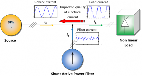
Figure 1 shows the block diagram of the shunt active filtering system.
Figure 1. Block diagram of shunt active filtering system
The main role of the insertion of the Shunt Active Power Filter is to produce currents against harmonics with the aim of compensating the harmonic currents generated by the non-linear load [4, 5]. Several methods are used for the identification of harmonics current such as Synchronous Reference Frame (SRF) theory and the instantaneous active and reactive power theory also called p-q method, the latter will be used in our case. the reference current is transmitted to a PWM control for the purpose of generated a switching signal to a two-level inverter which will subsequently supply the harmonic compensation current. The principle of SAPF is as shown in Figure 2.
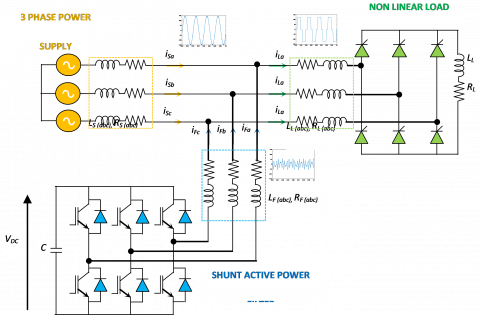
Figure 2. The basic principle of shunt active power filter
The instantaneous active and reactive power theory as shown in Figure 3 is used to the identification of harmonic currents. Akagi et al. [6] introduced this theory also called “p-q theory”, the concept of which consists of a variable transformation, in the α-β frame of reference, of the instantaneous powers, currents and voltages of the a-b-c frame [7].
Figure 3. Instantaneous active and reactive power theory
The transformed equations from three-phase plane to second with two-phase coordinates are given by the following equations.
$\left[v_{S}\right]=\left[\begin{array}{l}v_{S a} \\ v_{S b} \\ v_{S c}\end{array}\right]$ and $\left[i_{L}\right]=\left[\begin{array}{l}i_{L a} \\ i_{L b} \\ i_{L c}\end{array}\right]$ (1)
$\left[\begin{array}{l}v_{S \alpha} \\ v_{S \beta}\end{array}\right]=\sqrt{\frac{2}{3}}\left[\begin{array}{ccc}1 & -1 / 2 & -1 / 2 \\ 0 & \sqrt{3} / 2 & -\sqrt{3} / 2\end{array}\right]\left[\begin{array}{l}v_{S a} \\ v_{S b} \\ v_{S c}\end{array}\right]$ (2)
$\left[\begin{array}{c}i_{L \alpha} \\ i_{L \beta}\end{array}\right]=\sqrt{\frac{2}{3}}\left[\begin{array}{ccc}1 & -1 / 2 & -1 / 2 \\ 0 & \sqrt{3} / 2 & -\sqrt{3} / 2\end{array}\right]\left[\begin{array}{l}i_{L a} \\ i_{L b} \\ i_{L c}\end{array}\right]$ (3)
This transformation says of Concordia transformation is only valid if the voltage components are sinusoidal and balanced. The calculation of the instantaneous active and reactive powers in this reference is by:
$p=v_{S \alpha} \cdot i_{L \alpha}+v_{S \beta} \cdot i_{L \beta}$ (4)
$q=v_{S \alpha} \cdot i_{L \beta}-v_{S \beta} \cdot i_{L \alpha}$ (5)
From Eqns. (4) and (5), p and q can be expressed in AC and DC components, such as:
$p=\bar{p}+\tilde{p}$ (6)
$q=\bar{q}+\tilde{q}$ (7)
where, $\bar{p}:$ DC component of $p$ related to the classical fundamental active current; $\tilde{p}: \mathrm{AC}$ component, related to the harmonic currents caused by the alternative real instantaneous power; $\bar{q}: \mathrm{DC}$ component of $q$ related to the reactive power; $\tilde{q}$ : $\mathrm{AC}$ component, related to the harmonic currents caused by the alternative reactive power.
The currents in the $\alpha-\beta$ plane are given by the expression:
$\left[\begin{array}{l}i_{L \alpha} \\ i_{L \beta}\end{array}\right]=\frac{1}{v_{S \alpha}^{2}+v_{S \beta}^{2}}\left\{\left[\begin{array}{cc}v_{S \alpha} & v_{S \beta} \\ v_{S \beta} & -v_{S \alpha}\end{array}\right]\left[\begin{array}{l}p \\ 0\end{array}\right]\right.$
$\left.+\left[\begin{array}{cc}v_{S \alpha} & v_{S \beta} \\ v_{S \beta} & -v_{S \alpha}\end{array}\right]\left[\begin{array}{c}0 \\ q\end{array}\right]\right\}$
$=\left[\begin{array}{l}i_{L \alpha p} \\ i_{L \beta p}\end{array}\right]+\left[\begin{array}{l}i_{L \alpha q} \\ i_{L \beta q}\end{array}\right]$ (8)
To calculate the reactive power as well as the harmonic currents, the reference currents are calculated by:
$\left[\begin{array}{l}i_{F \alpha}^{*} \\ i_{F \beta}^{*}\end{array}\right]=\frac{1}{v_{S \alpha}^{2}+v_{S \beta}^{2}}\left[\begin{array}{cc}v_{S \alpha} & v_{S \beta} \\ v_{S \beta} & -v_{S \alpha}\end{array}\right]\left[\begin{array}{c}\tilde{p} \\ \bar{q}+\tilde{q}\end{array}\right]$ (9)
With the exception of the zero-sequence components, and in frame a-b-c, the active filter currents are:
The PI controller is used to get a stable and continuous voltage source to the inverter.
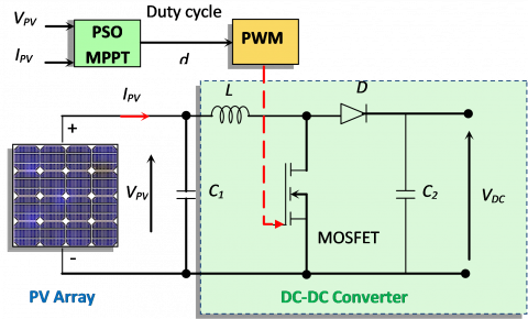
The photovoltaic system is used to supply a DC voltage source to the inverter. It consists of a photovoltaic field connected to a boost chopper [8] to reach a sufficient voltage. The control of the MOSFET is controlled by the MPPT technique. Figure 4 clearly indicate this assembly.
Figure 4. Photovoltaic system structure
4.1 The PV array
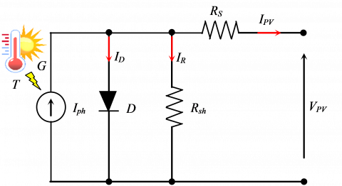
The PV Array is a linked set of photovoltaic modules in our work we will use the SunPower SPR-76R-BLK-U, each photovoltaic (PV) module is made up of several interconnected photovoltaic cells. The cells convert solar energy into direct current electricity, as shown in Figure 5, The mathematical modeling of the photovoltaic cell as a current source with an anti-parallel diode associated with series and parallel resistors [9, 10].
Figure 5. The equivalent model of PV cell
The equivalent circuit mathematical expression of the PV module is on Eq. (11):
$I_{P V}=I_{p h}-I_{D}-I_{R}$ (11)
$I_{P V}=I_{p h}-I_{0}\left[e^{q\left(\frac{V_{P V}+Z \cdot R_{S} \cdot I_{P V}}{z \cdot n \cdot k \cdot T_{c k}}\right)}-1\right]$
$-\frac{V_{P V}+Z \cdot R_{s} \cdot I_{P V}}{Z \cdot R_{s h}}$ (12)
where, $I_{P V}$ : Current (A), $I_{p h}$ : Photo-current (A), $I_{0}$ : Reverse saturation current $(\mathrm{A}), q$ : Electron charge $\left(1.602 \times 10^{-19}\right.$ Coulomb), $V$ : Voltage $(\mathrm{V}), z:$ Number of cells in series, $R_{s}$ : Series resistance $(\Omega), R_{s h}$ : Shunt resistance $(\Omega), n$ : Ideality factor varies between 1 and 2. $k$ : Boltzmann's constant $\left(1.381 \times 10^{-23} \mathrm{~J} / \mathrm{K}\right)$.
4.2 The particle swarm optimization
Onwubolu and Clerc [11] developed the popular stochastic optimization technique, called PSO. Figure 6 gives the approach of this method.
Figure 6. Flowchart of PSO algorithm [12]
4.3 The PSO-MPPT
The search for the favorable duty cycle which corresponds to the good global position of the ith particle is ensured by the PSO algorithm. First, the choice of the duty cycle applied at random to calculate the first particle. Then, the combined photovoltaic power is calculated using the measured output parameters such as photovoltaic current and voltage.
The value obtained is named pbest i and will be stored. By comparing the current value with the previous one, if this value is better, the algorithm will update it. Otherwise, don't change.
Similarly, the power value obtained will be compared with the best overall power value by this algorithm. If he gives us a better result, he will be convoluted by the new best overall position value. If all particles are tested, this action will end.
Then, the modification of position and speed will affect all the particles and as shown in Figure 7, these steps will be reproduced until obtaining the criterion of convergence, which describes all the steps of this algorithm. In the search space of the problem, the random arrangement of each particle is done at the start of the PSO algorithm.
The particles are moved by each iteration according to three components [2, 12]:
- At iteration k, the current velocity, $v_{i}^{k}$ is the best position of particle i;
- pbest and the best position,
- its gbest neighbors.
Figure 7. PSO-MPPT algorithm flowchart
Using MATLAB/Simulink, the model was developed. Table 1 shows the system parameter values.
Table 1. Simulation settings
|
Settings |
Numerical values |
|
|
Power network |
RMS voltage ES |
230 V |
|
Frequency f |
50 Hz |
|
|
Line resistor RS |
0.1 Ω |
|
|
Line Inductor LS |
0.03 mH |
|
|
Non-linear load (Rectifier) |
Load inductor NL LF |
0.3 mH |
|
Linear load |
Load resistor RL |
4 Ω |
|
Load inductor LL |
25 mH |
|
|
Load capacitor CL |
470 μF |
|
|
Active Parallel Filter PSO |
Filter inductor LFA |
1.3 mH |
|
The acceleration constants C1, C2 The inertia weight of particle w Nb of practice Nb of iteration |
1.2, 2 0.4 03 10 |
|
The Figure 8 shows the source currents waveform distorted and degraded by the nonlinear loads and before SAPF insertion.
Figure 8. Three-phases source current waveform before SAPF insertion
The Figure 9 shows the Total Harmonic Distorsion (THD) of a current source before SAPF insertion which displays 24.06%.
Figure 9. The THD of the current source before SAPF insertion
The Figure 10 shows the voltage delivered by the photovoltaic field which takes its maximum value of 312 V at 0.25 s.
Figure 10. The PV voltage Vpv
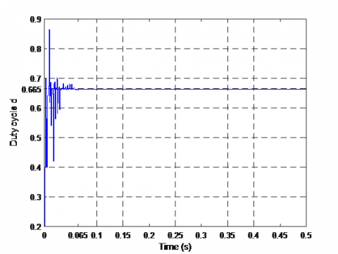
The Figure 11 shows the duty cycle d resulting at 0.065 s before calculating the best value from the PSO-MPPT method.
Figure 11. The duty cycle d
The Figure 12 shows the form of the Vdc voltage generate by the PV system and ameliorate by the PI controller.
Figure 12. The voltage Vdc delivered by the PV system
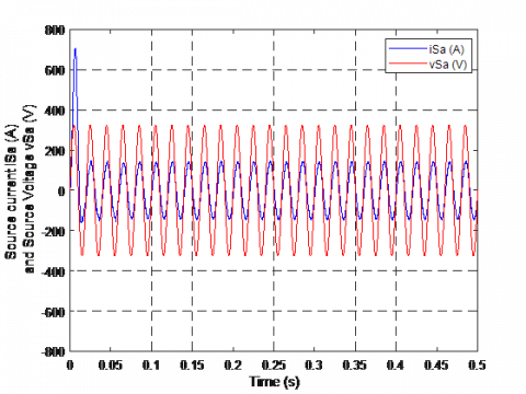
The Figure 13 shows the current and voltage which are in phase and we can clearly see that the source current isa becomes sinusoidal as well as the improvement of the power factor (0.0006 s, therefore φ=10.8°, that is to say a cosφ=0.98).
Figure 13. The waveform of the source current iSaand the source voltage vSa
The Figure 14 shows the source currents waveform after SAPF insertion.
Figure 14. The source currents waveform after SAPF insertion
The Figure 15 shows the Total Harmonic Distortion (THD) of a source current after SAPF insertion which displays 2.49%.
Figure 15. The THD of the source current after SAPF insertion
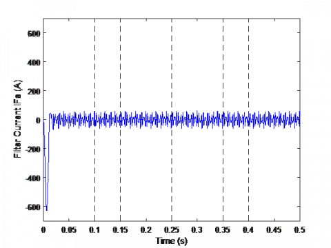
The Figure 16 shows the filter current iFa generate by the inverter.
Figure 16. The Filter current iFa
The Figure 17 shows the waveform of the load, filter and source currents iLa, iFa and iSa.
Figure 17. The Load iLa, the Filter iFa and the Source iSa currents
In this article, the modeling and simulation with MATLAB/Simulink of a SAPF supplied by photovoltaic system controlled with the particle swarm optimization algorithm gives good correction of power factor and harmonic distortion by providing cleanly sinusoidal current, and the application of the PSO algorithm has presented a high convergence speed, high precision, and it can accurately track the actual maximum power compared to conventional methods perturb and observe (P&O) and Incremental Conductance (IncCond).
We observe that the SAPF has been well filtered the current of line "a" which gives a THD of isa 2.49% after being 24.06% before application the SAPF. This result effectively meets the standards of IEEE-519 1992.
Through the positive results we have obtained, most electricity distribution institutions and even consumers are encouraged to adopt this technology in reducing pollution resulting from the use of non-linear load.
At the end of this study, we hope that we have given a view of the importance of filtering the electrical network. So, active filtering protects devices against malfunctions on one side, and filters power lines on the other side. To deepen this subject, we suggest an experimental study to validate the results obtained in practice.
We thank all the authors involved in this paper. Our thanks are essentially still aimed at all the teams of our research laboratories who have provided us with the means of preparing this article.
|
Abreviations |
|
|
p |
active power, W |
|
q |
reactive power, VAR |
|
D |
Duty cycle |
|
MPPT |
Maximum Power Point Tracking |
|
PSO |
Particle Swarm Optimization |
|
SAPF |
Shunt Active Power Filter |
|
THD |
Total Harmonic Distorsion |
|
Greek symbols |
|
|
$\alpha$ |
reference fram of $\alpha$ axe |
|
$\beta$ |
reference fram of $\beta$ axe |
|
$\phi$ |
solid volume fraction |
|
φ |
angle between current and voltage |
|
Subscripts |
|
|
s |
sourcee |
|
f |
filter |
|
l |
load |
|
pv |
photovoltaic |
|
s |
series |
|
sh |
dhunt |
|
ph |
Photo-current |
|
Constant values |
|
|
q |
Electron charge (1.602×10⁻¹⁹ Coulomb) |
|
k |
Boltzmann’s constant (1.381×10⁻²³J/K) |
|
n |
Ideality factor varies between 1 and 2 |
|
z |
Number of cells in series |
[1] Soto, E.A., Arakawa, K., Bosman, L.B. (2022). Identification of target market transformation efforts for solar energy adoption. Energy Reports, 8: 3306-3322. https://doi.org/10.1016/j.egyr.2021.12.043
[2] Ishaque, K., Salam, Z., Amjad, M., Mekhilef, S. (2012). An improved particle swarm optimization (PSO)–based MPPT for PV with reduced steady-state oscillation. IEEE transactions on Power Electronics, 27(8): 3627-3638. https://doi.org/10.1109/TPEL.2012.2185713
[3] Chao, K.H., Chang, L.Y., Liu, H.C. (2013). Maximum power point tracking method based on modified particle swarm optimization for photovoltaic systems. International Journal of Photoenergy, 2013. https://doi.org/10.1155/2013/583163
[4] Berbaoui, B., Benachaiba, C., Youcef, M. (2011). Power quality enhancement using shunt active power filter based on particle swarm optimization. Journal of Applied Sciences, 11(22): 3725-3731. https://doi.org/10.3923/jas.2011.3725.3731
[5] Chaoui, A., Gaubert, J.P., Bouafia, A. (2013). Direct power control switching table concept and analysis for three-phase shunt active power filter. Journal of Electrical Systems, 9(1): 52-65.
[6] Akagi, H., Hirokazu, W.E., Aredes, M. (2017). Instantaneous power theory and applications to power conditioning. IEEE Press, Wiley-Interscience, A John Wiley & Sons, Inc., Publication. https://doi.org/10.1002/9781119307181
[7] Manasa, P., Rao, K.N., Bhaskar, D.B. (2018). Mitigation of harmonics using shunt active power filter in the distribution system. Journal of Emerging Technologies and Innovative Research (JETIR), 5(7): 1513-1519. https://doi.org/10.46501/IJMTST061115
[8] IEEE Recommended Practices and Requirements for Harmonics Control in Electrical Power Systems IEEE 519-1992, IEEE Std., 1992.
[9] Almi, M.F., Arrouf, M., Belmili, H., Bendib, B. (2012). Contribution to the protection of PVG connected to three phase electrical network supply.
Energy Procedia, 18: 954-965. https://doi.org/10.1016/j.egypro.2012.05.110
[10] Areola, R.I., Oyediji, F.T., Olajuyin, E.A. (2021). Photovoltaic (PV) model evaluation with maximum power point tracking (MPPT). Journal of Engineering Research and Reports, 21(2): 1-8. https://doi.org/10.9734/JERR/2021/v21i217440
[11] Onwubolu, G.C., Clerc, M. (2004). Optimal path for automated drilling operations by a new heuristic approach using particle swarm optimization. International Journal of Production Research, 4: 473-491. https://doi.org/10.1080/00207540310001614150
[12] Kumar, A., Pant, S., Ram, M., Singh, S.B. (2017). On solving complex reliability optimization problem using multi-objective particle swarm optimization. Mathematics Applied to Engineering, pp. 115-131. https://doi.org/10.1016/B978-0-12-810998-4.00006-5