Younes Azzoug* | Remus Pusca | Mohamed Sahraoui | Abdelkarim Ammar | Tarek Ameid | Raphael Romary | Antonio J. Marques Cardoso
© 2021 IIETA. This article is published by IIETA and is licensed under the CC BY 4.0 license (http://creativecommons.org/licenses/by/4.0/).
OPEN ACCESS
This paper proposes a fault-tolerant control technique against current sensors failure in direct torque controlled induction motors drives, based on a new modification of Luenberger observer for currents estimation and axes transformation for vector rotation. Several important aspects are covered in the proposed algorithm, such as the detection of sensors failure, the isolation of faulty sensors, and the reconfiguration of the control system by a correct estimation. A logic circuit ensures fault detection by analyzing the residual signal between the measured and estimated quantities, while a single observer performs the task of estimating the line currents. In addition, a decision logic circuit isolates the erroneous signal and simultaneously selects the appropriate estimated current signal. An axes transformation ensures rotation from (a,b) to (α,β), which keeps a low-cost control using only two current sensors. The proposed scheme is tested on MATLAB/Simulink environment and experimentally validated in a laboratory prototype mainly containing a dS1104 card and 4 kW induction motor.
direct torque control, fault-tolerant control, fault detection, induction motor drive, current estimation
Fault Tolerant Control (FTC) methods are crucial in variable speed drives used in critical and high-sensitivity applications, such as, space exploration, nuclear power plants, electric vehicles, air and rail transportation; in order to ensure system security, and uninterrupted operation, even with degraded performance, when an unexpected failure occurs in the variable speed drive. Consequently, a fault tolerant control strategy must be implemented to guarantee that faults are handled in such a way that there will be no damage.
Generally, variable speed Induction Motor (IM) drives need feedback information from a speed/position transducer, two or three current sensors and a dc-link voltage sensor at least [1], [2]. Unfortunately, sensors are very prone to failures, and for this reason several research results have been published regarding sensors fault-tolerant control, as well as Fault Detection, Isolation, and Reconfiguration (FDIR) methods [3-10].
The study [3] presents a sensor FTC of an induction motor drive, based on the extended Kalman filter, and a reduced number of adaptive observers, to keep the operation of the system under the occurrence of sensors failures. In [4], a fault-tolerant vector control is proposed. A logic circuit is used to identify the faulty current sensor. The missing current information is replaced by an appropriate stator current, which value is calculated from algebraic equations and from the other measured healthy currents. However, this approach is not practical in the event of a successive failure in the different sensors. A fault-tolerant control scheme is proposed in Ref. [5], in which an adaptive fuzzy logic-based observer is used to generate residuals, which analysis allows the detection, and isolation of the faulty sensor. However, the dynamic response of this scheme for isolating defective sensors is too slow. In Ref. [6], it is proposed a sensor fault detection and isolation scheme for an IM drive, based on currents estimation and rotor resistance variations, which are then used in a decision unit for the identification and isolation of the faulty sensor. According to Yu et al. [7], a FTC technique against speed and current sensors failures in IM drives is proposed, and based on three adaptive observers with different inputs. However, this method is not suitable to achieve an efficient FTC in case of failures in two or three sensors. The results obtained by Yu et al. [8] offer a solution to the succession of faults in the different sensors but the number of the used adaptive observers is still three. Another type of FTC methods has been also presented in the literature, in which the sensors FTC algorithm changes the control according to the type of the faulty sensor, as proposed in Refs. [11-14]. A smooth FTC of IM drives with sensor failures is presented in the works [11, 12]. In the healthy state, the IM drive's operation is accomplished using direct torque control; indirect field-oriented control is then used when the dc-link voltage sensor fails, and v/f control is utilized during current sensors failure. The major drawback of this method, as reported by Tabbache et al. [15], is that these techniques are experimentally difficult to implement.
This paper proposes a direct torque fault-tolerant control strategy for the current sensor’s failure in induction motor drives. Some features are distinct from the other proposed methods. First, the estimation of stator currents is performed using a single observer. Then, the method proposed here allows the detection of faulty sensors even when several sensors fail successively, case in which a decision unit, based on a logic circuit, performs the task of reconfiguring and isolating the effects corresponding to the faulty sensor. Finally, the proposed technique can be reorganized in an adaptive way in the event of the loss of one or two sensors. The proposed scheme is simulated in MATLAB/Simulink environment, and experimentally implemented in a laboratory test bench under different operating conditions.
The remainder of the paper is organized into 5 sections. Section 2 analyses the direct torque control. Afterwards, section 3 describes the concept of the proposed FTC. Simulation and experimental results are presented and discussed in section 4. Finally, section 5 presents the main conclusion of the paper.
The system equation below gives the induction motor model used in the present work.
{disαdt=−(RsσLs+RrσLr)isα−ωrisβ+RsσLsLrψsα+ωrσLrψsβ+1σLsVsαdisβdt=−(RsσLs+RrσLr)isβ−ωrisα+RsσLsLrψsβ+ωrσLrψsα+1σLsVsβdψsαdt=Vsα−Rsisαdψsβdt=Vsβ−Rsisβ (1)
where:
Vsα,Vsβ:(α,β) stator voltages,
isα,isβ:(α,β) stator currents,
ψsα,ψsβ:(α,β) stator fluxes,
Rs,Rr : stator and rotor resistances,
Ls,Lr: stator and rotor inductances,
ωr : rotor angular speed.
σ=1−M2LsLr , given that M is the mutual inductance.
The electromagnetic torque is expressed by the following equation:
Te=p(ψsαisβ+ψsβisα) (2)
The stator flux components are given in the system equation below:
{ψsα=∫(Vsα−Rsisα)dtψsβ=∫(Vsβ−Rsisβ)dt (3)
The Direct Torque Control (DTC) basic idea is to estimate flux and torque instantaneous values only from the stator variables. The estimated torque is compared with the reference one given by the speed controller (PI controller in the present work), the resulting torque error signal is sent to a hysteresis controller (three-levels hysteresis controller is adopted in the present work) to get a control signal CTe, which fed a switching look-up table. Likewise, to the estimated flux, which is compared with fixed value of a stator flux magnitude, the resulting flux error signal is fed an hysterisis controller (two-levels hysterisis controller is adopted in the present work) to get a control signal Cflx for the switchin look-up table. This latter uses flux and torque control signals in order to generate three control signals SA,SB and SC for the three-phase inverter (see Figure 4).
In the proposed fault-tolerant direct torque control, two current sensors in phase-a, and phase-b are used in addition to a dc-link voltage sensor, and an incremental encoder. Furthermore, using the control signals SA, SB and SC, a voltage synthesizer constructs the three-phase stator voltages applied to the machine from the voltage measured in the dc-link.
3.1 Stator currents estimation
In order to estimate the line currents, a modified adaptive observer is used, which gives high-performance estimation stator currents, based on the IM model, which is described by the following state equation:
{˙X=A(ωr)X+BUY=CX (4)
here:
X=[isαisβψrαψrβ]T;Y=[isαisβ]TU=[VsαVsβ]T
and:
A=[a10a2ωra30a1−ωra3a2a40a5−ωr0a4ωra5];B=[1σLs001σLs0000];C=[10000100]
as well as:
a1=−(1τsσ+(1−σ)τrσ);a2=MσLsLrτr;a3=MσLsLr;a4=Mτr;a5=1τr;τs=LsRs;τr=LrRr;
The idea of the proposed stator currents estimator is based on the general theory of Luenberger observer [16], which allows the estimation of variable or unknown parameters of a system. The equation of the Luenberger observer is expressed in (5), where the symbol “^” denotes the estimated values:
{˙ˆX=A(ωr)ˆX+BU+KξˆY=CˆX (5)
where:
ˆX=[^lsα^lsβ^ψrα^ψrβ]T;ˆY=[^lsα^lsβ]T;ξ=[isα−^lsαisβ−^lsβ]T
Since there is no information about the measured currents, the vector ξ becomes:
ξ=[−^lsα−^lsβ]T
The estimation is performed throw the conservation of the state model (4) of the IM with the gain matrix K. This matrix ensures the convergence of the observer, and has been determined by the classical pole placement procedure. Then, replacing the adaptive mechanism by the measured rotational speed, as well as, feeding the observer with the stator voltages provided by the voltage synthesizer. This gives the stator currents estimation, as illustrated in Figure 1.
Figure 1. Proposed stator currents estimator
Considering the following system of equations, that present the current observer model in the complex format, the gain matrix K is defined as follows:
{˙ˉX=ˉAˆX+BˉVs+ˉKξˆY=CˆˉX (6)
The determination of the gain matrix K uses the conventional pole placement procedure, through the imposition of the observer's poles and consequently of its dynamics [17-20].
The characteristic equation of the observer is as follow:
G(s)=det(sI−(ˉA−ˉKC)) (7)
Developing the different matrices A, K and C knowing that ˉK=[K′K′′] the following equation is obtained:
G(s)=s2+(1σTs+1σTr−jωr+K′)s+(1Tr−jωr){(1σTs+1σTr)+K′}+(MTr−K′′)(MσLsLr)(1Tr−jωr) (8)
where, K' and K'' are complex gains.
The dynamic equation of the observer is defined as:
H(s)=s2+l(1σTs+1σTr−jωr)s+l2(1Tr−jωr){(1σTs+1σTr)}+(MTr)(MσLsLr)(1Tr−jωr) (9)
where, l is the proportionality constant, slightly bigger than the unit (l=1.004).
Eqns. (8) and (9) are in the form of the following equation:
HP(s)=s2+2εωns+ω2n (10)
The comparison of Eqns. (8) and (9) gives for the expressions of K' and K'':
{K′=(l−1)(1σTs+1σTr−jωr)K′′=(l−1)[{[1σTs+1σTr]σLsMLr−MTr}(l+1)−σLsMLr[1σTs+1σTr]+jωrσLsMLr] (11)
To get the gain matrix K it is supposed that:
{K′=K1+jK2K′′=K3+jK4 (12)
So,
K1=(l−1)(1στs+1στr)K2=−(l−1)ωrK3=(l2−1)[(1στs+1στr)σLsMLr−Mτr]+σLsMLr(1στs+1στr)(l−1)K4=−(l−1)σLsMLrωr
According to the anti-symmetry of matrix A, the gain matrix K is set as follows:
K=[K1K2K3K4−K2K1−K4K3]T
3.1.1 Currents estimator stability
Considering the following equations:
Induction motor model: ˙X=AX+BU (13)
and
Observer model: ˙ˆX=AˆX+BU+Kξ (14)
The estimated stator currents error (e=IS−ˆIS) is the deference between the observer and the induction motor models, so:
˙e=(A−KC)e (15)
Considering the Lyapunov function below:
S=eTe+(Δωr)2λ (16)
Its time derivative is:
dSdt=(deTdt)e+(dedt)eT+1λddt(Δωr)2 (17)
Knowing that Δωr=0 , then:
dSdt=(deTdt)e+(dedt)eT (18)
Replacing Eq. (15) in Eq. (18) gives:
dSdt=e{(A−KC)T+(A−KC)}eT (19)
A sufficient condition for this estimator stability is that Eq. (19) is equal to zero, and indeed, this equation is always equal to zero.
3.2 Fault detection, isolation and system reconfiguration
The logic-circuit presented in Figure 2 is intended to ensure the fault detection, isolation, and system reconfiguration. The detection of failures is performed by analyzing the residual signal between the measured and estimated quantities, passing through a Low Pass Filter (LFP) to extract the useful signal that will be compared to a well-defined threshold (Th=0.8), then a proper estimation is used for the isolation and reconfiguration of the system.
Figure 2. Fault detection, isolation and system reconfiguration scheme
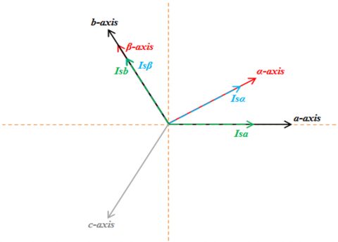
As mentioned previously, two current sensors (in phase-a and phase-b) were used in the proposed method for measuring a and b line currents. The axis transformation presented in Figure 3 developed by Chakraborty and Verma [21] and used in both [22, 23], which is also used in the proposed FTC, in order to have the component currents (α,β) using only the measurements of (a, b) components.
Figure 3. Axis transformation model
As shown in Figure 3, the β-axis is aligned with the b-axis. Considering the equation of transformation from (a, b) to (α,β), which is given in (20), it is clear that isα depends on the two-phase currents Isa and Isb, whereas the current isβ depends only on the current Isb. Therefore, if the phase-a current sensor becomes faulty, only iSα that will be affected. But, if the phase-b current sensor becomes faulty, both currents isα and isβ will be affected.
[isαisβ]=[2/√31/√301][IsaIsb] (20)
So, the faulty measured current components (α,β) must be replaced by the corresponding estimated currents. As a consequence, Table 1 shows the identification of the faulty sensors and the correct components of the estimated currents that will replace the erroneous components.
Table 1. Faulty sensor identification and correct component selection
|
Sensor-a |
Sensor-b |
Za |
Zb |
OR |
Proper selected components |
|
Healthy |
Healthy |
0 |
0 |
0 |
isα mes and isβ mes |
|
Faulty |
Healthy |
1 |
0 |
1 |
isαest and isβ mes |
|
Healthy |
Faulty |
0 |
1 |
1 |
isα est and isβ est |
|
Faulty |
Faulty |
1 |
1 |
1 |
isαest and isβest |
As presented in Figure 2 and defined in Table I, it appears that in the case of sensor-a failure, fault detection part of the logic circuit generates an impulse Za=1, whereas, in the case of sensor-b failure, fault detection logic circuit generates an impulse Zb=1. Once the faulty sensor is identified, it is isolated, and the system is reconfigured, using the fault isolation and system reconfiguration part of the logic circuit. The logic gate OR output is 1 when any one of its inputs Za or Zb or both is 1 due to the effect of the failure of sensor-b on isα current. As a consequence, in the case of sensor-b failure, isα mes is isolated and replaced by isa est.
The proposed current sensor direct torque fault-tolerant control for induction motor drive is simulated in Matlab\Simulink environment using 4 kW induction motor parameters (see the Appendix). Figure 4 presents the block diagram of the proposed method.
Figure 4. Block diagram of the proposed FTC
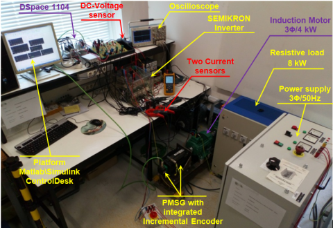
Figure 5 displays the laboratory test bench in which the proposed control technique has been implemented and tested experimentally, which is composed mainly of a 4 kW three-phase IM whose parameters are the same used in simulation model, dS1104 card, two current sensors, and dc-voltage sensor.
Figure 5. Laboratory experimental test bench
All simulation and experimental tests are performed at 1000 rpm with 20 N.m load torque.
4.1 Test of the proposed FTC when sensor-a becomes faulty and sensor-b remains healthy
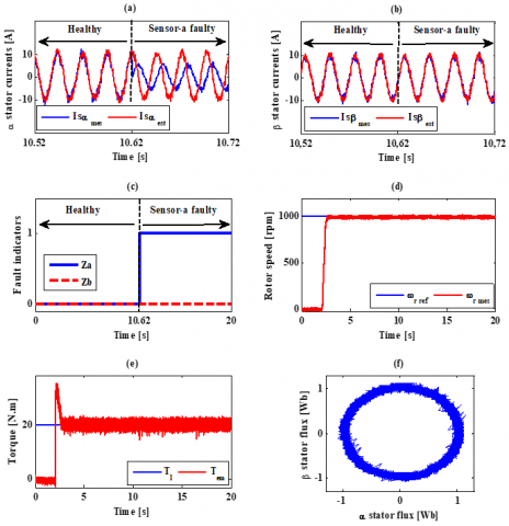
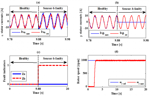
Figures 6 and 7 show simulation and experimental results obtained respectively, applying the proposed FTC. The drive was started with healthy current sensors in both simulation and experimentation. At t=1 s in simulation test and t=10.6 s in experimental test, current sensor-a fails. As a result and corresponding to the used axis transformation equation (6), isα mes becomes faulty such is depicted in Figures 6(a) and 7(a), and isβ mes remains healthy as can be seen in Figures 6(b) and 7(b). At the moment of failure occurrence, Za sensor-a state indicator becomes 1, judging sensor-a faulty, but Zb sensor-b state indicator remains 0, affirming that sensor-b is healthy, as illustrated in Figures 6(c) and 7(c). As a consequence of Za=1, switch-a switches to input 1 to replace the erroneous measured current by the estimated one as explained previously in Table 1. Figures 6(d), 7(d) and 6(e), 7(e) illustrate respectively the high-performance speed tracking of the IM drive, and the uninterrupted fulfillment of electromagnetic torque requirement under both healthy and faulty conditions, and Figures 6(f), 7(f) depict stator flux circular trajectory.
Figure 6. Simulation results when sensor-a is faulty and sensor-b remains healthy: (a) isα currents, (b) isβ currents, (c) fault indicator, (d) reference and actual speeds, (e) load and electromagnetic torque, and (f) stator flux trajectory
Figure 7. Experimental results when sensor-a is faulty and sensor-b remains healthy: (a) isα currents, (b) isβ currents, (c) fault indicator, (d) reference and actual speeds, (e) load and electromagnetic torque, and (f) stator flux trajectory
4.2 Test of the proposed FTC when sensor-b becomes faulty and sensor-a remains healthy
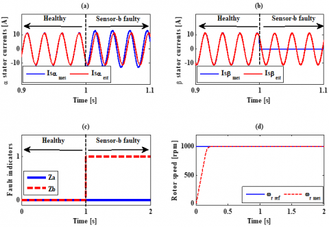
Figures 8 and 9 give another test of the suggested FTC method with simulation and experimentation respectively, where a failure in sensor-b is performed, whereas sensor-a remains healthy. Simulation and experimental tests were started in healthy conditions until t=1 s for simulation test and t=9.8 s for experimental test, where sensor-b becomes faulty. Considering Figures 8(a) and 9(a), it can be seen that isα mes is slightly affected by the failure of sensor-b, while isβ mes is significantly affected, which is explained previously in Eq. (6). The fault detection algorithm reacts quickly by generating an impulse Zb=1, indicating that sensor-b is faulty, unlike Za which remains at 0, meaning that sensor-a gives proper measurement. At this moment, switch-b switches to input 1 to replace isβ mes by isβ est , and according to the output of the gate OR (see Table 1) switch-a switches to input 1 to replace isα mes by isα est . Figures 8(c) and 9(c) demonstrate sensor state indicators Za and Zb. Figures 8(d) for simulation and 9(d) for experimentation show the speed tracking performance of the IM drive before and after the failure occurrence.
Figure 8. Simulation results when sensor-b is faulty and sensor-a remains healthy: (a) isα currents, (b) isβ currents, (c) fault indicator, and (d) reference and actual speeds
Figure 9. Experimental results when sensor-b is faulty and sensor-a remains healthy: (a) isα currents, (b) isβ currents, (c) fault indicator, and (d) reference and actual speeds
4.3 Test of the proposed FTC when both sensor-a and sensor-b become faulty
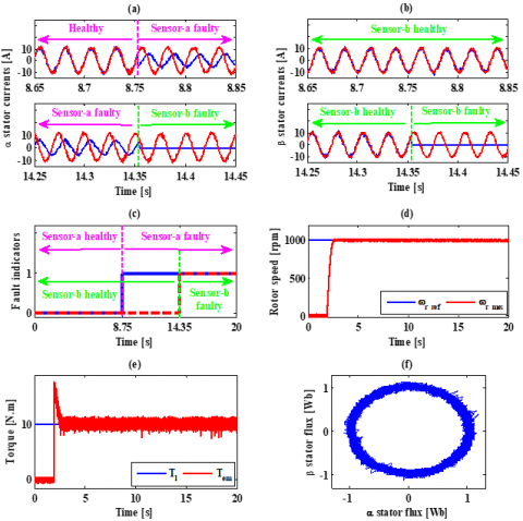
Figures 10 and 11 illustrate respectively the simulation and experimentation results obtained by applying the proposed FTC when the both sensors fail. The sensor-a failure is simulated at t=1s, while the sensor-b fault is simulated at t=1.1 s as shown in the Figures 10(a) and 10(b). In the experimental test, sensor-a failure is appeared at t=8.75 s, while sensor-b failure is appeared at t=14.35 s as can be seen in Figures 11(a) and 11(b). While, Figures 10(c) and 11(c) show the fault indicator signals (Za for sensor-a and Zb for sensor-b). When the defect is suddenly introduced in the sensor-a, the fault detection mechanism has reacted quickly by generating a Za index equal to 1, indicating that sensor-a is faulty. Based on Eq. (6), the current isβ mes will not be affected, which is visible in Figures 10(b) and 11(b), where the current isβ mes remains healthy from 0 to 1.1 s in simulation and until 14.34 s in experimentation. According to Table 1, the selected currents to isolate the faulty measurement are: isα est and isβ mes. After 1.1s in simulation and 14.35s in experimentation, a fault has been introduced in sensor-b, at this moment, the fault indicator Zb becomes 1, confirming sensor-b failure. Referring to equation (6), we can see that the currents isα and isβ both depend on the state of the measurment of sensor-b, which is confirmed in Figures 10(a) and 11(a) where the degree of severity of the fault in the current isα mes is increased. Therefore, the isolation and reconfiguration algorithm choose isα est and isβ est (see Table 1).
Figure 10. Simulation results when both sensor-a and sensor-b become faulty: (a) isα currents, (b) isβ currents, (c) fault indicator, (d) reference and actual speeds, (e) load and electromagnetic torque, and (f) stotor flux trajectory
Figure 11. Experimental results when both sensor-a and sensor-b become faulty: (a) isα currents, (b) isβ currents, (c) fault indicator, (d) reference and actual speeds, (e) load and electromagnetic torque, and (f) stotor flux trajectory
Figures 10(d), 11(d) and 10(e), 11(e) clearly show that speed and torque maintain their performance and remain uninterrupted, even under the worst possible conditions, when the both current sensors fail. In addition, Figures 10(f) and 11(f) show the constant estimate of stator flux.
This paper presents a direct torque fault-tolerant control diagram for current sensors failures in the induction motor drives. For the identification of a sensor failure, a logic circuit is used in the phases where the current sensors are located, which is able to detect the failures of the used current sensors. A current estimator is used to estimate the stator currents. Immediately after the failure of the current sensor, a decision logic circuit automatically selects the correct current signal to maintain the operation of the system. Simulation and experimental results show the effectiveness of the proposed method, where the fault detection is accomplished with fast dynamics, and the drive is performing successfully, without compromising the control system.
This work has been achieved within the framework of CE2I project (Convertisseur d’Energie Intégré Intelligent). CE2I is co-financed by European Union with the financial support of the European Regional Development Fund (ERDF), French State and the French Region of Hauts-de-France.
As well, this work was supported by the European Regional Development Fund (ERDF) through the Operational Program for Competitiveness and Internationalization - COMPETE 2020, and also by National Funds through the Portuguese Foundation for Science and Technology (FCT), under Project POCI-01-0145-FEDER-029494 and Project UID/EEA/04131/2013.
|
IM |
Induction Motor |
|
DTC |
Direct Torque Control |
|
FTC |
Fault Tolerant Control |
|
FDIR |
Fault Detection, Isolation and Reconfiguration |
|
PMSG |
Permanent Magnet Synchronous Generator |
|
AC |
Alternative Current |
|
DC |
Direct Current |
|
Vdc |
DC-link voltage |
|
Vs |
Three phases stator voltages |
|
Ia,Ib,Ic |
Three phases stator currents |
|
Vsα,Vsβ |
(α,β) axis stator voltages |
|
Isα,Isβ |
(α,β) axis stator currents |
|
φsα,φsβ |
(α,β) axis stator fluxes |
|
φrα,φrβ |
(α,β) axis rotor fluxes |
|
φr |
Rotor flux magnitude |
|
ωS |
Synchronous speed |
|
ωr |
Rotor angular speed |
|
ωe |
Electrical angular speed |
|
Ωr |
Mechanical speed |
|
Te,Tl |
Electromagnetic and load torques |
The used induction motor specifications and parameters:
|
Specifications |
Parameters |
||
|
Nominal power [kW] |
4 |
Rs [Ω] |
1.5 |
|
Nominal voltage [V] |
400 |
Rr [Ω] |
2.03 |
|
Nominal current [A] |
9.2 |
Ls [H] |
0.36 |
|
Frequency [Hz] |
50 |
Lr [H] |
0.36 |
|
Number of pole pairs |
2 |
M [H] |
0.35 |
|
Nominal speed [rpm] |
1415 |
J [Kg.m2] |
0.024 |
|
|
|
f [Nm.s.rad-1] |
0.002 |
[1] Berriri, H., Naouar, M.W., Slama-Belkhodja, I. (2011). Easy and fast sensor fault detection and isolation algorithm for electrical drives. IEEE Transactions on Power Electronics, 27(2): 490-499. https://doi.org/10.1109/TPEL.2011.2140333
[2] Yu, Y., Chen, X., Dong, Z. (2017). Current sensorless direct predictive control for induction motor drives. In 2017 IEEE Transportation Electrification Conference and Expo, Asia-Pacific (ITEC Asia-Pacific) pp. 1-6. https://doi.org/10.1109/ITEC-AP.2017.8080975
[3] Zhang, X., Foo, G., Don Vilathgamuwa, M., Tseng, K.J., Bhangu, B.S., Gajanayake, C. (2013). Sensor fault detection, isolation and system reconfiguration based on extended Kalman filter for induction motor drives. IET Electric Power Applications, 7(7): 607-617. https://doi.org/10.1049/iet-epa.2012.0308
[4] Dybkowski, M., Klimkowski, K. (2016). Stator current sensor fault detection and isolation for vector controlled induction motor drive. In 2016 IEEE International Power Electronics and Motion Control Conference (PEMC), pp. 1097-1102. https://doi.org/10.1109/EPEPEMC.2016.7752147
[5] Lee, K.S., Ryu, J.S. (2003). Instrument fault detection and compensation scheme for direct torque controlled induction motor drives. IEE Proceedings-Control Theory and Applications, 150(4): 376-382. https://doi.org/10.1049/ip-cta:20030596
[6] Najafabadi, T.A., Salmasi, F.R., Jabehdar-Maralani, P. (2010). Detection and isolation of speed-, DC-link voltage-, and current-sensor faults based on an adaptive observer in induction-motor drives. IEEE Transactions on Industrial Electronics, 58(5): 1662-1672. https://doi.org/10.1109/TIE.2010.2055775
[7] Yu, Y., Wang, Z., Xu, D., Zhou, T., Xu, R. (2014). Speed and current sensor fault detection and isolation based on adaptive observers for IM drives. Journal of Power Electronics, 14(5): 967-979. https://doi.org/10.6113/JPE.2014.14.5.967
[8] Yu, Y., Zhao, Y., Wang, B., Huang, X., Xu, D. (2017). Current sensor fault diagnosis and tolerant control for VSI-based induction motor drives. IEEE Transactions on Power Electronics, 33(5): 4238-4248. https://doi.org/10.1109/TPEL.2017.2713482
[9] Mendes, A.M., Cardoso, A.M. (2006). Fault-tolerant operating strategies applied to three-phase induction-motor drives. IEEE Transactions on Industrial Electronics, 53(6): 1807-1817. https://doi.org/10.1109/TIE.2006.885137
[10] Azzoug, Y., Menacer, A., Pusca, R., Romary, R., Ameid, T., Ammar, A. (2018). Fault tolerant control for speed sensor failure in induction motor drive based on direct torque control and adaptive stator flux observer. In 2018 International Conference on Applied and Theoretical Electricity (ICATE), pp. 1-6. https://doi.org/10.1109/ICATE.2018.8551478
[11] Stettenbenz, M., Liu, Y., Bazzi, A. (2015). Smooth switching controllers for reliable induction motor drive operation after sensor failures. In 2015 IEEE Applied Power Electronics Conference and Exposition (APEC), pp. 2407-2411. https://doi.org/10.1109/APEC.2015.7104685
[12] Liu, Y., Stettenbenz, M., Bazzi, A.M. (2018). Smooth fault-tolerant control of induction motor drives with sensor failures. IEEE Transactions on Power Electronics, 34(4): 3544-3552. https://doi.org/10.1109/TPEL.2018.2848964
[13] Sepe, R.B., Morrison, C., Miller, J.M. (2003). Fault-tolerant operation of induction motor drives with automatic controller reconfiguration. Practical Failure Analysis, 3(1): 64-70. https://doi.org/10.1109/IEMDC.2001.939291
[14] Aguilera, F., Pablo, M., De Angelo, C.H. (2015). A fault tolerant system for current sensors in induction motor drives. In 2015 XVI Workshop on Information Processing and Control (RPIC), pp. 1-7. https://doi.org/10.1109/RPIC.2015.7497178
[15] Tabbache, B., Rizoug, N., Benbouzid, M.E.H., Kheloui, A. (2012). A control reconfiguration strategy for post-sensor FTC in induction motor-based EVs. IEEE Transactions on Vehicular Technology, 62(3): 965-971. https://doi.org/10.1109/TVT.2012.2232325
[16] Luenberger, D. (1971). An introduction to observers. IEEE Transactions on Automatic Control, 16(6): 596-602. https://doi.org/10.1109/TAC.1971.1099826
[17] Keller, H. (1987). Non-linear observer design by transformation into a generalized observer canonical form. International Journal of Control, 46(6): 1915-1930. https://doi.org/10.1080/00207178708934024
[18] Leu, Y.G., Lee, T.T., Wang, W.Y. (1999). Observer-based adaptive fuzzy-neural control for unknown nonlinear dynamical systems. IEEE Transactions on Systems, Man, and Cybernetics, Part B (Cybernetics), 29(5): 583-591. https://doi.org/10.1109/3477.790441
[19] Kubota, H., Sato, I., Tamura, Y., Matsuse, K., Ohta, H., Hori, Y. (2002). Regenerating-mode low-speed operation of sensorless induction motor drive with adaptive observer. IEEE Transactions on Industry Applications, 38(4): 1081-1086. https://doi.org/10.1109/TIA.2002.800575
[20] Miklosovic, R., Radke, A., Gao, Z. (2006). Discrete implementation and generalization of the extended state observer. In 2006 American Control Conference, pp. 6-pp. https://doi.org/10.1109/ACC.2006.1656547
[21] Chakraborty, C., Verma, V. (2014). Speed and current sensor fault detection and isolation technique for induction motor drive using axes transformation. IEEE Transactions on Industrial Electronics, 62(3): 1943-1954. https://doi.org/10.1109/TIE.2014.2345337
[22] Manohar, M., Das, S., Kumar, R. (2017). A robust current sensor fault detection scheme for sensorless induction motor drive. In 2017 IEEE PES Asia-Pacific Power and Energy Engineering Conference (APPEEC), pp. 1-6. https://doi.org/10.1109/APPEEC.2017.8308967
[23] Manohar, M., Das, S. (2017). Current sensor fault-tolerant control for direct torque control of induction motor drive using flux-linkage observer. IEEE Transactions on Industrial Informatics, 13(6): 2824-2833. https://doi.org/10.1109/TII.2017.2714675