Seif-El Islam Chelli* | Ahmed Lokmane Nemmour | Mourad Ait Ahmed | Abdelfettah Boussaid | Abdelmalek Khezzar
© 2020 IIETA. This article is published by IIETA and is licensed under the CC BY 4.0 license (http://creativecommons.org/licenses/by/4.0/).
OPEN ACCESS
When using the forgetting factor recursive least squares (FF-RLS) method for a real-time identification of the squirrel-cage induction motor parameter's purposes, the main difficulty encountered is that the rotor state variables are not accessible for measurements. This fact involves supplementary computations under some controverted simplifying assumptions and yields to an over-parameterizing algebraic model. For the doubly fed induction machine configuration, many recent works presented in literature persist to use this method in an identical manner in spite of the fact that all rotor’s quantities are available for this machine’s conception. This work deals with the presentation of a new approach based on the RLS method with a forgetting factor especially designed for on-line parameter's estimation relative to the doubly fed induction machine case. Hence, by knowing the ratio between the stator and the rotor windings voltages respectively that is performed in the no-load transformer test; the studied situation will be treated as any linear time invariant system parameters identification with no adopted restrictions. The effectiveness of the suggested alternative is confirmed experimentally with improved estimation characteristics.
doubly fed induction machines, squirrel-cage induction machine, real-time parameters estimation, forgetting factor recursive least-squares algorithm (FF-RLS)
Due to their well-known intrinsic advantages with respect to other kinds of electrical machines, Induction machines continue to be considered as the most important element in all industrial mechanisms and drives [1]. In other hand, these benefits are associated to some disagreeable facts characterizing these actuators traduced principally by complex mechanical and electromagnetic behaviors characterizing the transient machine operating conditions. In addition, nonlinearity, high coupling terms and some time-varying parameters will appear in the different mathematical models describing these systems.
In electrical drives and power-generation, applications based induction machines; an accurate determination of the parameters characterizing these electromechanical converters has a major task, especially in cases where the values of these parameters are needed to dimensioning the various closed-loop controllers, estimators and observers algorithms [2-4]. Traditionally, the determination of these parameters values is made by realizing a specific laboratory experiment. However, the obtaining parameters accuracy depends essentially on the class of different devices used for the measure, the machine size and experimentation conditions. The wanted parameters value that figure in several input-output transfer functions could be also determined by performing some appropriate frequency responses tests. Nevertheless, this procedure is not suitable due to corresponding practical tests restrictions [5].
In order to have a better way to determine the parameters of the induction machine, innovative approaches consist essentially in performing a recursive form concerning the unknown machine parameters values and the instantaneous machine signals available for measure. These quantities are principally the stator voltage terminals, the stator winding currents and the mechanical speed. The real-time form of these techniques constitutes an efficient solution especially when the considered machine is operating under some practical constraints such as the main core saturation and heating effects. In this way, several real-time parameters estimation approaches were presented in literature [6-10].
For the wound-rotor induction machine case, an estimation procedure based on the least-squares method using the starting transient data is presented by Kojooyan-Jafari et al. [11]. However, the described algorithm is applied in a same way of a squirrel-cage induction machines and requiring first and second derivation computations. The considered approach [12] consists in performing parameters estimation algorithm when the considered machine is operating under vector control conditions including closed loops regulations via PI controllers. Better results could be obtained under supplementary computations relative to the control structure requirements. Another off-line solution uses a quadritization method by making approximation through a quadratic polynomial interpolation is discussed by Hasni et al. [13], However the presented approach requires an additional computation based on frequency responses to determine the rotor time constant. More efficient techniques use the well-known Lyapunov stability theory to synthesize an adaptive law of the MRAS method [14]. Nevertheless, the exciting signals must be selected in order to obtain a significant response of all dynamical system eigenvalues.
The Forgetting factor Recursive Least-Squares (FF-RLS) method is surely one of the best-recommended approaches for the real-time system parameters identification [15]. Since this technique offers a fast convergence speed, it constitutes a powerful tool for real-time process parameters identification especially in the case of systems with no large matrixes [16, 17]. During these last decades, many varieties of recursive least-squares algorithms were developed for the real-time induction machine parameters identification. When using the RLS technique to define the parameters values characterizing an induction machine mathematical model, it is recommended to formulate the state-space machine model in two orthogonal axes related to the rotor or the stator reference frames. The procedure frequently adopted is to transform the original dynamical machine model into a linear parameterized form where figure the stator voltage vector and its first derivative, the stator current vector, it first and second derivatives and the shaft velocity which is commonly treated as a slowly changing quantity. In this new form, the resulting stationary coefficients represent in fact a linear or nonlinear combination of the desired machine parameters [18-22]. Therefore, this obtained parameterized model is executed simultaneously with the physical machine and the unknown model parameters are on-line estimated by decreasing the error between the machine and this developed model outputs [23].
The present work discusses with application of a conventional variant of the FF-RLS algorithm to a specific doubly fed induction machine dynamical model intentionally developed for an on-line electrical machine parameters identification. Therefore, considering the fact that the rotor currents are available for measure, the introduced machine model is ready to a direct use of the FF-RLS algorithm by avoiding the first derivative of stator voltage and the second derivative of stator current computations generally required for the squirrel-cage machines configuration. Moreover, the real-time identification procedure is carried out with no limitations about the rotor speed profile. These vital benefits offer precise on-line parameter’s estimation independently of the operating conditions.
This paper begins by describing the conventional method applied for the induction machine parameters estimation using the forgetting factor recursive least squares (FF-RLS) method. In the third section, a new dynamical model exclusively performed for doubly fed induction machine. According to the previous FF-RLS algorithm requirements, this model is adapted and rearranged into a linear parameterized form. Simulation tests are presented in the fourth section to verify the proposed method validity. A comparative study with the conventional procedure relative to the squirrel-cage induction machine is given. Finally, an experimental verification using a dSpace-1104 controller board is carried-out.
2.1 Induction motor linear parameterized form
The following part deals with the presentation of a linear form frequently employed for real-time induction machine parameters estimation by the FF-RLS algorithm. So, an induction motor could be modeled by the following equations set relative to the stationary (a,b) reference frame:
$\left\{\begin{array}{l}\bar{V}_{s}=R_{s} \bar{I}_{s}+\dot{\bar{\phi}} \\ \bar{V}_{r}=R_{r} \bar{I}_{r}+\dot{\bar{\phi}}_{r}-j \omega \phi_{r} \\ \frac{J}{p M} \dot{\omega}=\operatorname{Imag}\left(\bar{I}_{r} \times \bar{I}_{s}\right)-\frac{B}{p} \omega-\tau_{L}\end{array}\right.$ (1)
where,
$\left\{ \begin{array}{*{35}{l}}{{{\bar{V}}}_{s}}={{v}_{s\alpha }}+j{{v}_{s\beta }} \\ {{{\bar{I}}}_{s}}={{i}_{s\alpha }}+j{{i}_{s\beta }} \\ {{{\bar{I}}}_{r}}={{i}_{r\alpha }}+j{{i}_{r\beta }} \\\end{array} \right.$ (2)
By taking into account that the rotor flux and currents could not be measured for the squirrel-cage machines case, it is necessary to derive the next linear parameterized form without any rotor quantities:
$\left[\begin{array}{cccc}\dot{I}_{s} & \bar{I}_{s} & -j \omega \bar{I}_{s} & -\dot{\bar{V}}_{s}+j \omega \bar{V}_{s} & -\bar{V}_{s}\end{array}\right]$
$\left[\begin{array}{l}\theta_{1} \\ \theta_{2} \\ \theta_{3} \\ \theta_{4} \\ \theta_{5}\end{array}\right]=\left[-\ddot{\bar{I}}_{s}+j \omega \dot{\bar{I}}_{s}-j \dot{\omega} \beta \dot{\bar{\phi}}_{r}\right]$ (3)
The stator quantitites in (1) and the angular rotor speed are available for measure. A detailed demonstration of (3) is given in the study [17]. When the motor is operating at fixed speed, then $\dot{\omega}=0$, in this case, (3) will be reduced to:
$\left[\begin{array}{cccc}\dot{\bar{I}} & \bar{I}_{s} & -j \omega \bar{I}_{s} & -\dot{\bar{V}}_{s}+j \omega \bar{V}_{s} & -\bar{V}_{s}\end{array}\right]$ (4)
The standard linear form given by (5) could represent Eq. (4):
$Y=U \theta^{\prime}$ (5)
where,
$\left\{\begin{array}{l}Y=\left[-\ddot{I}_{s}+j \omega \dot{\bar{I}}_{s}\right] \\ U=\left[\dot{\bar{I}}_{s} \bar{I}_{s}-j \omega \bar{I}_{s}-\dot{\bar{V}}_{s}+j \omega \bar{V}_{s}-\bar{V}_{s}\right] \\ \theta=\left[\frac{1}{\sigma T_{s}}+\frac{\beta_{0}}{\sigma} \frac{\beta_{0}}{\sigma T_{s}} \frac{1}{\sigma T_{s}} \frac{1}{\sigma L_{s}} \frac{\beta_{0}}{\sigma L_{s}}\right]\end{array}\right.$ (6)
With $\beta_{0}=\frac{R_{r}}{L_{r}}=\frac{1}{T_{r}}$.
One remark that the following relation could associate the θ- elements:
$\theta_{2} \theta_{4}=\theta_{3} \theta_{5}$ (7)
The parameters $\theta$ define the following machine parameters Rs, Ls, σ and Tr as:
$\left\{\begin{array}{l}R_{s}=\frac{\theta_{2}}{\theta_{5}}=\frac{\theta_{3}}{\theta_{4}} \\ L_{s}=\frac{\theta_{1}-\theta_{3}}{\theta_{5}} \\ T_{r}=\frac{\theta_{4}}{\theta_{5}} \\ \sigma=\frac{\theta_{5}}{\theta_{4}\left(\theta_{1}-\theta_{3}\right)}\end{array}\right.$ (8)
2.2 The FF-RLS parameters identification algorithm
In order to achieve a complete FF-RLS algorithm formulation, (5) can be rewritten as:
$\left[\begin{array}{llll}u_{1}(n) & u_{2}(n) & \dots & u_{n}\end{array}\right]\left[\begin{array}{llll}\theta_{1} & \theta_{2} & \dots & \theta_{n}\end{array}\right]^{\prime}=U \theta^{\prime}=Y(u)$ (9)
By considering some external disturbances relative to the measured quantities, the output of (9) could be rewritten as:
$y(n)=U \hat{\theta}=\hat{\varepsilon}(n)$ (10)
where, $\hat{\theta}$ denotes the identified values of the system vector parameters and $\hat{\varepsilon}$ is the model prediction error.
From (9) and (10), this modeling error can be evaluated as follows:
$\hat{\varepsilon}(n)=U(\theta-\hat{\theta})$ (11)
By selecting an adequate performance function J, based on the square prediction error defined as:
$J=\sum_{i=1}^{N} \hat{\varepsilon}_{i}^{2}=\hat{\varepsilon} \hat{\varepsilon}^{\prime}$ (12)
The unknown system parameters constitute the solution of the following equation:
$\frac{\partial J}{\partial \theta}=0$ (13)
From the two above equations, the desired solution is expressed as:
$\theta=\left[U U^{\prime}\right]^{-1}[U \theta]$ (14)
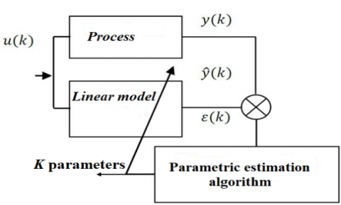
Figure 1 illustrates the real-time estimation layout describing the forgetting factor recursive least squares (FF-RLS) method.
Figure 1. Real-time identification parameters model based on the FF-RLS algorithm
Detailed algorithm steps explaining the standard FF-RLS method are presented in appendix A.
Eq. (4) was derived to satisfy the FF-RLS method requests. This convenient form is obtained by considering that the rotor velocity has a fixed value. Despite this simplifying supposition, this form requires some complex calculations such as the first and second derivatives of stator current, and the first derivative of stator voltage vector.
In the following paragraph, the suggested induction machine dynamical model is detailed. The corresponding linear parameterized form is obtained with no assumptions made about the rotor speed dynamics. In addition, just the first derivative of the stator current is necessary to perform the proposed on-line parameter's estimation.
3.1 The wound-rotor induction machine dynamical model derivation
By referring to the unmoving reference frame, the induction machine behavior is entirely traduced by (1). Therefore, the stator and rotor fluxes vector $\bar{\phi}_{s}$ and $\bar{\phi}_{r}$ are expressed in terms of the stator and rotor currents vectors as follows:
$\left\{\begin{array}{l}\bar{\phi}_{s}=L_{s} \bar{I}_{s}+M \bar{I}_{r} \\ \bar{\phi}_{r}=M \bar{I}_{s}+L_{r} \bar{I}_{r}\end{array}\right.$ (15)
Then the differentiation of these two fluxes quantities gives:
$\left\{\begin{array}{l}\dot{\bar{\phi}}_{s}=L_{s} \dot{\bar{I}}_{s}+M \dot{\bar{I}}_{r} \\ \dot{\bar{\phi}}_{s}=L_{r} \dot{\bar{I}}_{r}+M \dot{\bar{I}}_{s}\end{array}\right.$ (16)
According to Eqns. (15) and (16), (1) becomes:
$\left\{ \begin{array}{*{35}{l}} {{{\bar{V}}}_{s}}={{R}_{s}}{{{\bar{I}}}_{s}}+{{L}_{s}}{{{\dot{\bar{I}}}}_{s}}+M{{{\dot{\bar{I}}}}_{r}} \\ \begin{align} & 0={{R}_{r}}{{{\bar{I}}}_{r}}+{{L}_{r}}{{{\dot{\bar{I}}}}_{r}}+M\dot{\bar{I}}-j\omega \left( {{L}_{r}}{{{\bar{I}}}_{r}}+M{{{\bar{I}}}_{s}} \right) \\
& \frac{J}{pM}\dot{\omega }=Imag\left( {{{\bar{I}}}_{r}}\times {{{\bar{I}}}_{s}} \right)-\frac{B}{p}\omega -{{\tau }_{L}} \\ \end{align} \\\end{array} \right.$ (17)
The principal goal is to rewrite this model in a new form where appear only the desired parameters Rs, Ls, $\sigma$ and Tr. For this reason (17) will be modified as follows:
$\left\{ \begin{array}{*{35}{l}} {{{\bar{V}}}_{s}}={{R}_{s}}{{{\bar{I}}}_{s}}+{{L}_{s}}{{{\dot{\bar{I}}}}_{s}}+M\left( \frac{M}{{{L}_{r}}} \right)\left( \frac{{{L}_{r}}}{M} \right){{{\dot{\bar{I}}}}_{r}} \\ \begin{align} & 0={{R}_{r}}\left( \frac{M}{{{L}_{r}}} \right)\left( \frac{{{L}_{r}}}{M} \right){{{\bar{I}}}_{r}}+{{L}_{r}}\left( \frac{M}{{{L}_{r}}} \right)\left( \frac{{{L}_{r}}}{M} \right){{{\dot{\bar{I}}}}_{r}}+M{{{\dot{\bar{I}}}}_{s}}-j\omega \left( {{L}_{r}}\left( \frac{M}{{{L}_{r}}} \right)\left( \frac{{{L}_{r}}}{M} \right){{{\bar{I}}}_{r}}+M{{{\bar{I}}}_{s}} \right) \\ & \frac{J}{pM}\dot{\omega }=Imag\left( \left( \frac{M}{{{L}_{r}}} \right)\left( \frac{{{L}_{r}}}{M} \right){{{\bar{I}}}_{r}}\times {{{\bar{I}}}_{s}} \right)-\frac{B}{p}\omega -{{\tau }_{L}} \\ \end{align} \\
\end{array} \right.$(18)
By adopting the variable changing given by:
$\vec{I}_{r}=\left(\frac{L_{r}}{M}\right) \bar{I}_{r}$ (19)
Eq. (18) becomes:
$\left\{\begin{array}{l}\bar{V}_{s}=R_{s} \bar{I}_{s}+L_{s} \dot{\bar{I}}_{s}+\left(\frac{M^{2}}{L_{r}}\right) \dot{\bar{I}}_{r}^{\prime} \\ 0=\left(\frac{R_{r}}{L_{r}}\right) \bar{I}_{r}^{\prime}+\dot{\bar{I}}_{r}^{\prime}+\dot{\bar{I}}_{s}-j \omega\left(\bar{I}_{r}^{\prime}+\bar{I}_{s}\right) \\ \frac{J}{p} \dot{\omega}=\left(\frac{M^{2}}{L_{r}}\right) \operatorname{Imag}\left(\bar{I}_{r}^{\prime} \times \bar{I}_{s}\right)-\frac{B}{p} \omega-\tau_{L}\end{array}\right.$ (20)
The ratio $\frac{L_{r}}{M}$ necessary for performing the mentioned variable changing constitutes an unknown quantity. However, for the slip ring induction machine configuration, it characterizes the ratio between the stator and rotor terminal voltages; it is measured by performing the no-load transformer test.
Since the desired parameters are interrelated as follows:
$\left\{\begin{array}{l}T_{r}=\frac{L_{r}}{R_{r}} \\ \frac{M^{2}}{L_{r}}=(1-\sigma) L_{s}\end{array}\right.$ (21)
where, $\sigma$ defines the leakage factor, it is associated to cyclic machine inductances as:
$\sigma=1-\frac{M^{2}}{L_{r} L_{s}}$ (22)
Finally, the following condensed form could represent the resulting wound-rotor induction machine mathematical model as:
$\bar{V}_{s}=R_{s} \bar{I}_{s}+L_{s} \dot{\bar{I}}_{s}+(1-\sigma) L_{s} \dot{\bar{I}}^{\prime}$ (23)
$0=\frac{1}{T_{r}} \bar{I}_{r}^{\prime}+\dot{\bar{I}}_{r}^{\prime}+\dot{\bar{I}}_{s}-j \omega\left(\bar{I}_{r}^{\prime}+\bar{I}_{s}\right)$ (24)
$\frac{J}{p} \dot{\omega}=\operatorname{Imag}\left(\bar{I}_{r}^{\prime} \times \bar{I}_{s}^{*}\right)(1-\sigma) L_{s}-\frac{B}{p} \omega-\tau_{L}$ (25)
From the previous model, one can conclude that the identifiable parameters $R_{s}, L_{s}, \sigma$ and $T_{r}$ are satisfactory to describe entirely the induction machine mathematical model regardeless of its rotor construction.
3.2 A model of the wound-rotor induction machine in a linearized form
In (23), the stator voltage space vector contains both stator and rotor currents first derivatives. By substituting the rotor current expression given by (24) into (23), the two next equivalent formulations with just one rotor or stator currents differentiation could be obtained:
$\bar{V}_{s}=R_{s} \bar{I}_{s}+j L_{s} \omega\left(\bar{I}_{r}^{\prime}+\bar{I}_{s}\right)-\frac{L_{s}}{T_{r}} \bar{I}_{r}^{\prime}+\sigma L_{s} \dot{\bar{I}}_{s}^{\prime}$ (26)
$\bar{V}_{s}=R_{s} \bar{I}_{s}+j(1-\sigma) L_{s} \omega\left(\bar{I}_{r}^{\prime}+\bar{I}_{s}\right)-\frac{(1-\sigma) L_{s}}{T_{r}} \bar{I}_{r}^{\prime}+\sigma L_{s} \dot{\bar{I}}_{s}^{\prime}$ (27)
In the case where (26) is maintained, then it could be rearranged under the following way:
$\left[\bar{V}_{s}\right]=\left[\bar{I}_{s}-j \omega\left(\bar{I}_{r}^{\prime}+\bar{I}_{s}\right)-\bar{I}_{r}^{\prime}-\dot{\bar{I}}_{r}^{\prime}\right]\left[R_{s} \quad L_{s} \frac{L_{s}}{T_{r}} \sigma L_{s}\right]^{\prime}$ (28)
This matrix expression represents is identical to (5) which is given by:
$Y=U \theta^{\prime}$ (29)
With:
$\left\{\begin{array}{l}Y=[\bar{V}] \\ U=\left[\bar{I}-j \omega\left(\bar{I}_{r}+\bar{I}_{s}\right)-\bar{I}^{\prime}-\dot{I}^{\prime}\right] \\ \theta=\left[R_{s} L_{s} \frac{L_{s}}{T_{r}} \sigma L_{s}\right]\end{array}\right.$ (30)
In this situation, the output vector Y is constituted by the stator voltages when the input vector U is represented by the stator and rotor currents and the mechanical speed acquisitions. Nevertheless, it is indispensable to perform the rotor current component's differentiation. Here, The machine parameters $R_{s}, L_{s}, \sigma$ and $T_{r}$ to be identified will figure explicitly in the estimated vector θ elements:
$\left\{\begin{array}{l}R_{s}=\theta_{1} \\ L_{s}=\theta_{2} \\ T_{r}=\frac{\theta_{2}}{\theta_{3}} \\ \sigma=\frac{\theta_{4}}{\theta_{2}}\end{array}\right.$ (31)
It can be noticed that the proposed procedure given by (30) is practical and more convenient to identify a slip-rings induction machine than the standard one given by (6).
For the other model given by (27), a similar reasoning could be adopted. The linear formula will be given by :
$\bar{V}_{s}=\left[\begin{array}{llll}\bar{I}_{s} & j \omega\left(\bar{I}_{r}^{\prime}+\bar{I}_{s}\right) & \bar{I}_{r}^{\prime} & \dot{\bar{I}}_{s}^{\prime}\end{array}\right]\left[R_{s}(1-\sigma) L_{s} \frac{(1-\sigma) L_{s}}{T_{r}} \sigma L_{s}\right]$ (32)
Then the corresponding machine parameters are computed in the following way:
$\left\{\begin{array}{l}R_{s}=\theta_{1} \\ L_{s}=\theta_{2}+\theta_{4} \\ T_{r}=\frac{\theta_{2}}{\theta_{3}} \\ \sigma=\frac{\theta_{4}}{\theta_{2}+\theta_{4}}\end{array}\right.$ (33)
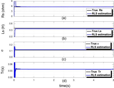
The proposed doubly fed induction machine parameters identification was initially verified by performing various standard identification tests to a laboratory wound-rotor induction motor prototype (Table 1). Hence, the measured parameters values that are taken as real values Rs_real, Ls_real Rs_true, Tr_real and $\sigma_{\text {real}}$ are used to configure a simulated wound rotor induction machine parameters where the stator windings are fed with a balanced three phase voltages source. During the simulation time range, the aim is to check the FF-RLS algorithm capacity to converge to the true parameters with a sampled time of 0.1ms during five seconds signals relative to the stator currents and voltages, rotor currents and the rotor speed. The simulated rotor speed during the starting and the transient measured stator currents waveforms are represented in Figure 2. The corresponding estimated parameters Rs, Ls, σ and Tr variations with respect to (30) are visualized in Figure 3 with their analogous true values.
Figure 2. Simulated waveforms:(a): Rotor speed, (b): $i_{s \beta}$, (c): $i_{s a}$
Figure 3. Real and estimated electrical parameters values:(a): RS, (b); Ls, (c): σ, and (d): Tr
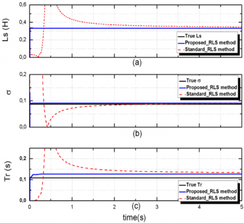
Figure 4. Comparison between estimated parameters using the proposed FF-RLS method, standard RLS method and true value:(a): LS, (b): σ and (c): Tr
Table 1. The used wound rotor induction motor data
|
Parameter description |
Values |
|
Rated power Prated [kW] |
220 |
|
Rated voltage Urated [V ] |
1.5 |
|
Rated frequency f [Hz] |
50 |
|
pole-pairs |
2 |
|
Stator resistance Rs [Ω] |
4 , 7 |
|
Stator inductance Ls [H] |
0,3949 |
|
Rotor resistance Rr [Ω] |
0 , 5 |
|
Rotor inductance Lr [H] |
0,023 |
|
Three-phase magnetizing Lm [H] |
0,0896 |
Table 2. Induction motor estimated parameters using the suggested algorithm
|
Machine parameters |
Trus values |
Estimate Values |
Percent errors |
|
Rs[Ω] |
4.7 |
4.6747 |
0.54 |
|
Ls[H] |
0.3949 |
0.3949 |
0.0 |
|
Tr[s] |
0.0460 |
0.04601 |
0.021 |
|
σ |
0.1161 |
0.1056 |
9.04 |
In order to examine the of the proposed FF-RLS doubly fed induction machine parameters estimation efficiency with respect to the standard one presented in section 2, a machine data cited by Vieira et al. [24] have been adopted. In Figure 4. The results relative to each procedure are compared. One can see that a better convergence of the estimated parameters is obtained.
Table 3 gives a comparison between the identified and true parameters values cited by Vieira et al. [24]; these later are considered as reference. The evaluation results indicate that the estimated parameters are perfectly tracked to their respective true values.
Concerning the parameters estimation robustness relative to the used RLS algorithm, simulation study is curried out: due to the heat effects, the stator and rotor resistances are intentionally increased with 20% with respect to their rated values presented in Table 4. Figure 5 shows that the adopted approach offers a good sensitivity according to the introduced parameters variations.
Table 3. The obtained parameters using the suggested algorithm
|
Machine parameters |
Trus values |
Proposed RLS |
Percent errors |
Standard RLS |
Percent errors |
|
Ls [H] |
0.335 |
0.335 |
0.0 |
0.348 |
3.88 |
|
Tr [s] |
0.109 |
0.127 |
16.51 |
0.134 |
22.94 |
|
$\sigma$ |
0.088 |
0.091 |
3.41 |
0.09 |
2.27 |
Table 4. Induction motor estimated parameters when the stator and rotor resistances are increased with 20%
|
Machine parameters |
Trus values |
Estimate Values |
Percent errors |
|
Rs[Ω] |
5.64 |
5.618 |
0.3901 |
|
Ls[H] |
0.3949 |
0.3949 |
0.0 |
|
Tr[s] |
0.0383 |
0.03832 |
0.052 |
|
σ |
0.1161 |
0.1056 |
9.04 |
Figure 5. Estimated parameters when the stator and rotor resistances are increased with 20%:(a):Rs, (b): LS, (c): σ and (d): Tr
In this part, experimental tests are performed in order to verify the aptitude of the proposed FF-RLS method to estimate parameters defining the studied wound-rotor induction motor by using the proposed approach. The obtained results are compared to the conventional ones that are qualified as the true values.
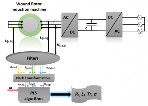
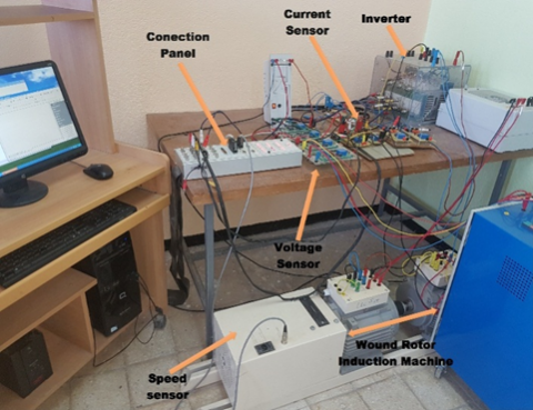
The proposed estimation doubly fed induction machine parameters procedure based on the FF-RLS strategy was executed via Dspace-DS1104 signal processor control card. For a concrete reason, the starting-up process is realized by a three-phase voltage source Semikron inverter. By adopting a sampling time of 0.1 ms, the mechanical speed is obtained from a 1024 incremental encoder resolution when the stator voltages and the stator and rotor windings currents are obtained from a voltage and current sensors respectively. In addition, appropriate anti-aliasing filters are used to accomplish the different signals discretization process [24-26]. Figure 6 and Figure 7 illustrate respectively the layout of the real-time parameter’s estimation method implemented in the Dspace card and the corresponding experimental test-bench.
Figure 6. Layout of real-time parameters estimation relative to the proposed FF-RLS method
Figure 7. Test Bench picture
Figure 8. Waveforms: (a): Rotor speed, (b): $\dot{l}_{s \beta}$, (c): $i_{s \alpha}$
Practically, the motor starts at t=0.6s, the corresponding shaft speed and the transient stator currents evolutions under no load conditions are shown in Figure 8.
Figure 9 indicates that the suggested FF-RLS technique offers a fast convergence of estimated parameters to their desired values.
In Table 5, is reported a comparison between the real values and the related parameters values with the proposed approach. By referring to these results, the real-time estimation parameters are accomplished with a good accuracy.
From the results presented in Table 2 and Table 5, it can be noticed, that errors between the obtained parameters in simulation and experimental tests, are partially related to the considered hypothesis in the simulation study. Here, the main source of these errors could be referred to the used algorithm itself. Others influencing factors could be associated to the hardware circuit’s elements such as the digital interfacing circuits components; current/voltage sensors intrinsic errors.
Figure 9. The estimated electrical parameters by the proposed RLS method: (a): Rs, (b): Ls, (c): σ and (d): Tr (experimental results)
Table 5. Parameters of the used induction motor
|
Machine parameters |
Trus values |
Estimate Values |
Percent errors |
|
Rs[Ω] |
4.7 |
4.93 |
4.88 |
|
Ls[H] |
0.3949 |
0.3925 |
0.608 |
|
Tr[s] |
0.0460 |
0.0547 |
18.91 |
|
σ |
0.1161 |
0.1080 |
6.97 |
In this paper, the popular forgetting factor recursive least-squares method is applied to a wound-rotor induction machine mathematical model especially developed for real-time electrical parameters estimation. Due to the developed model advantages, the online estimation process is realized with no complicated computations encountered in the squirrel-cage induction machine configuration. Furthermore, no limitations are imposed concerning to the rotor speed variation. These important benefits provide a quick and precise identification of parameters values in real time under steady state and transient conditions. The estimated parameters accuracy is evaluated by comparing the experimental results with the laboratory tests obtained from conventional tests. This comparison shows a good agreement. For future works, the obtained results could be improved using advanced estimation methods such us the stochastic RLS algorithm, the Kalman filtering algorithm, genetic algorithms and some so-called meta-heuristic methods.
|
$\bar{\phi}_{s}, \bar{\phi}_{r}$ |
stator flux vector and rotor flux vector |
|
$\bar{V}_{s}, \bar{V}_{r}$ |
stator voltage vector and rotor voltage vector |
|
$\bar{I}_{s}, \bar{I}_{r}$ |
stator current vector and rotor current space |
|
$R_{s}, R_{r}$ |
stator resistance and rotor resistance |
|
$L_{s}, L_{r}$ |
stator inductance and rotor inductance |
|
M |
mutual inductance |
|
$\tau_{L}$ |
load torque |
|
p |
number of pole pairs |
|
$\omega$ |
angular rotor speed |
|
$T_{r}$ |
rotor time constant |
|
$\sigma$ |
total leakage coefficient |
|
j |
the standard $\sqrt{-1}$ complex number |
APPENDIX
According to the RLS algorithm, this n components vector can be estimated iteratively by performing the following steps [27-29]:
1. The initial value of the estimated is set equal to zero $\hat{\theta}(0)=0_{n \times 1}$. However, a square covariance matrix P needed for the recursive process must also be initialized as a diagonal matrix with large positive diagonal numbers $P(0)=\alpha I_{n \times n}$,
2. The estimated output $\hat{y}$ can be evaluated by $\hat{y}(k)=u(k) \hat{\theta}^{\prime}(k-1)$, then the estimation error relative to the actual measured output system y is computed by $\varepsilon(k)=y(k)-\hat{y}(k)$
3. The covariance matrix can be updated according to the following expression as:
$P(k)=P(k-1)+\Delta P(k)$
With:
$\Delta P(k)=-\frac{P(k-1) u^{\prime}(k) u(k) P(k-1)}{\mu+u(k) P(k-1) u^{\prime}(k)}$
Usually forgetting factor µ$\in$[0.8, 1] but does not make the value too small, for it may reduce the accuracy of identification.
4. Finally, the actual value of the vector parameters $\hat{\theta}$ is estimated by $\hat{\theta}(k)=\hat{\theta}(k-1)+\Delta \hat{\theta}(k)$ with $\Delta \hat{\theta}(k)=P(k) u^{\prime}(k) \varepsilon(k)$
Repeat steps 2-4 until a preset minimum error ε (k) is reached.
[1] Imakiire, A., Lipo, T.A. (2019). Induction machine with localized voltage unbalance compensation. 2019 IEEE International Electric Machines & Drives Conference (IEMDC), San Diego, CA, USA, pp. 1248-1255. https://doi.org/10.1109/IEMDC.2019.8785168
[2] Krishnan, R. (2001). Electric Motor Drives: Modeling, Analysis, and Control. Prentice Hall.
[3] Leonhard, W. (2012). Control of Electrical Drives. Springer Science Business Media, 2012.
[4] Bouzid, M.B.K., Champenois, G., Tnani, S. (2018). Reliable stator fault detection based on the induction motor negative sequence current compensation. International Journal of Electrical Power Energy Systems 95: 490-498. https://doi.org/10.1016/j.ijepes.2017.09.008
[5] Vas, P. (1993). Parameter Estimation, Condition Monitoring, and Diagnosis of Electrical Machines. Oxford University Press.
[6] Tăut, M., Chindris, G., Pitică, D., Fodor, A. (2017). Model-in-the-loop for determining the parameters of a dc motor. 2017 IEEE 23rd International Symposium for Design and Technology in Electronic Packaging (SIITME), Constanta, pp. 267-273. https://doi.org/10.1109/SIITME.2017.8259906
[7] Zhan, X., Zeng, G.H., Liu, J., Wang, Q.Z., Ou, S. (2015). A review on parameters identification methods for asynchronous motor. International Journal of Advanced Computer Science and Applications, 6(1). https://dx.doi.org/10.14569/IJACSA.2015.060115
[8] Sim, H.W., Lee, J.S., Lee, K.B. (2014). On-line parameter estimation of interior permanent magnet synchronous motor using an extended Kalman filter. Journal of Electrical Engineering and Technology, 9(2): 600-608. https://doi.org/10.5370/JEET.2014.9.2.600
[9] Papadopoulos, T.A., Barzegkar-Ntovom, G.A., Nikolaidis, V.C., Papadopoulos, P.N., Burt, G.M. (2017). Online parameter identification and generic modeling derivation of a dynamic load model in distribution grids. 2017 IEEE Manchester PowerTech, Manchester, pp. 1-6. https://doi.org/10.1109/PTC.2017.7980994
[10] Morfín, O.A., Castañeda, C.E., Ruiz-Cruz, R., Valenzuela, F.A., Murillo, M.A., Quezada, A.E., Padilla, N. (2018). The squirrel-cage induction motor model and its parameter identification via steady and dynamic tests. Electric Power Components and Systems, 46(3): 302-315. https://doi.org/10.1080/15325008.2018.1445140
[11] Kojooyan-Jafari, H., Monjo, L., Córcoles, F., Pedra, J. (2014). Parameter estimation of wound rotor induction motors from transient measurements. IEEE Transactions on Energy Conversion, 29(2): 300-308. https://doi.org/10.1109/TEC.2014.2300236
[12] Leite, V., Araujo, R., Freitas, D. (2002). Flux and parameters identification of vector-controlled induction motor in the rotor reference frame. 7th International Workshop on Advanced Motion Control. Proceedings (Cat. No.02TH8623), Maribor, Slovenia, pp. 263-268. https://doi.org/10.1109/AMC.2002.1026928
[13] Hasni, M., Mancer, Z., Mekhtoubb, S., Bacha, S. (2012). Parametric identification of the doubly fed induction machine. Energy Procedia, 18: 177-186. https://doi.org/10.1016/j.egypro.2012.05.029
[14] Thomsen, S., Rothenhagen, K., Fuchs, F.W. (2014). Online parameter identification methods for doubly fed induction generators. 008 IEEE Power Electronics Specialists Conference, Rhodes, pp. 2735-2741. https://doi.org/10.1109/PESC.2008.4592358
[15] Wang, J. (2009). A variable forgetting factor RLS adaptive filtering algorithm. 2009 3rd IEEE International Symposium on Microwave, Antenna, Propagation and EMC Technologies for Wireless Communications, Beijing, pp. 1127-1130. https://doi.org/10.1109/MAPE.2009.5355946
[16] Tang, J., Yang, Y., Blaabjerg, F., Chen, J., Diao, J.L., Liu, Z.G. (2018). Parameter identification of inverter-fed induction motors: A review. Energies, 11(9): 2194. https://doi.org/10.3390/en11092194
[17] Robertson, D.G., Lee, J.H., (2002). On the use of constraints in least squares estimation and control. Automatica, 38(7): 1113-1123. https://doi.org/10.1016/S0005-1098(02)00029-8
[18] Elisei-Iliescu, C., Stanciu, C., Paleologu, C., Benesty, J., Anghel, C., Ciochină, S. (2017). Robust variable-regularized RLS algorithms. 2017 Hands-free Speech Communications and Microphone Arrays (HSCMA), San Francisco, CA, pp. 171-175. https://doi.org/10.1109/HSCMA.2017.7895584
[19] Stephan, J., Bodson, M., Chiasson, J. (1994). Real-time estimation of the parameters and fluxes of induction motors. IEEE Transactions on Industry Applications, 30(3): 746-759. https://doi.org/10.1109/28.293725
[20] Koubaa, Y. (2006). Asynchronous machine parameters estimation using recursive method. Simulation Modelling Practice and Theory, 14(7): 1010-1021. https://doi.org/10.1016/j.simpat.2006.07.003
[21] M., Cirrincione, M., Pucci, G., Cirrincione, G. Capolino, (2003). A new experimental application of least-squares techniques for the estimation of the induction motor parameters. IEEE Transactions on Industry Applications 39(5): 1247-1256. https://doi.org/10.1109/TIA.2003.816565
[22] Alkamachi, A. (2019). Permanent magnet DC motor (PMDC) model identification and controller design. Journal of Electrical Engineering, 70(4): 303-309. https://doi.org/10.2478/jee-2019-0060
[23] Debbabi, F., Nemmour, A.L., Khezzar, A., Chelli, S. (2020). An approved superiority of real-time induction machine parameter estimation operating in self-excited generating mode versus motoring mode using the linear RLS algorithm: Ideas & applications. International Journal of Electrical Power & Energy Systems, 118: 105725. https://doi.org/10.1016/j.ijepes.2019.105725
[24] Vieira, R.P., Azzolin, R.Z., Gastaldini, C.C., Grundling, H.A. (2010). Electrical parameters identification of hermetic refrigeration compressors with single-phase induction machines using RLS algorithm. The XIX International Conference on Electrical Machines - ICEM 2010, Rome, pp. 1-6. https://doi.org/10.1109/ICELMACH.2010.5607994
[25] Mitra, S.K., Kuo, Y. (2006). Digital Signal Processing a Computer-Based Approach. McGraw-Hill Higher Education New York.
[26] Guo, J.T., Li, G.L., Xie, F., Hu, C.G.., Pan, Z.F., Meng, N. (2014). On-line parameter identification of asynchronous motor using improved least squares. 2014 9th IEEE Conference on Industrial Electronics and Applications, Hangzhou, pp. 130-134. https://doi.org/10.1109/ICIEA.2014.6931145
[27] Diniz, P.S. (1997). Adaptive Filtering. Springer. https://doi.org/10.1007/978-1-4614-4106-9
[28] Hu, Y. (2013). Iterative and recursive least squares estimation algorithms for moving average systems. Simulation Modelling Practice and Theory, 34: 12-19. https://doi.org/10.1016/j.simpat.2012.12.009
[29] Djadi, H., Yazid, Y.K., Menaa, M. (2017). Parameters identification of a brushless doubly fed induction machine using pseudo-random binary signal excitation signal for recursive least squares method. IET Electric Power Applications, 11(9): 1585-1595. https://doi.org/10.1049/iet-epa.2017.0083