Hayder Gallas* | Amina Mseddi | Sandrine Le Ballois | Helmi Aloui | Lionel Vido
© 2020 IIETA. This article is published by IIETA and is licensed under the CC BY 4.0 license (http://creativecommons.org/licenses/by/4.0/).
OPEN ACCESS
Setting up an experimental test bench for a large-scale wind conversion system (WCS) could be very challenging in terms of cost, size and complexity of the electrical and mechanical components especially in an academic research environment. Therefore, the aim of this paper is to establish an alternative through the development of a realistic simulation model. Such a model is essential for a better performances’ assessment of the studied 1.5 MW aerogenerator, based on a Hybrid Excitation Synchronous Generator (HESG). A model of the WCS taking into account both complex electrical phenomena and aerodynamic behaviors is established using the code FAST. Two pitch controllers are proposed and investigated. The first one consists of a conventional PI regulator. As for the second one, it includes a PI-based fuzzy logic controller. The blades’ loads, the low-speed shaft (LSS) torque ripple and loads are also given. Simulations results have confirmed the efficiency of the implemented fuzzy logic pitch controller and the capabilities of the developed model in simulating the behaviors of the modeled WCS in different operating regions.
FAST, HESG, large-scale WCS, modeling, PI-based fuzzy logic control, robust control
In the last decade, wind energy has occupied a leading position among renewable energy resources with a cumulative global installed capacity of 539.6 GW worldwide in 2017 [1]. Besides, it presents one of the most promising forms of renewable energy regarding ecology, jobs creation and development potentials [2]. The operating of a wind turbine can be described by the variation of the generated power on its low-speed shaft as a response to the changes of the wind velocity, as illustrated in Figure 1.
Figure 1. Typical wind turbine power curve
It comprises, mainly, three operating regions (referred to as zone I to III):
In a WCS, the integrity of the aerogenerator structure is a significant factor so it can operate with an optimum energy production at a minimum cost. In the case of a large wind turbine, the risk associated with mechanical fatigue comes mainly from the torque ripple of the rotor shaft. This particular phenomenon is due to many factors such as the sudden changes in the wind velocity, the HESG space harmonics or the vibrations in the transmission system.
The considered WCS is based on a hybrid excitation synchronous generator (HESG) connected to an isolated load and a variable speed horizontal axis wind turbine.
The transmission system comprises a gearbox that connects the wind turbine-side low-speed shaft (LLS) to the generator-side high-speed shaft (HSS). The primary purpose of the gearbox is to convert the high torque low-speed rotational velocity generated by the turbine rotor into a low torque high-speed velocity feeding the HESG.
The flux created in the air gap of the HESG comes from two sources: permanent magnets mounted on the rotor and excitation coils on the stator (Figure 2). This hybrid excitation principle offers an additional degree of freedom allowing much flexibility in the control of the excitation flux. Furthermore, the topology of a HESG comes without slip rings or brushes.
In short, as explained by Vido et al. [3], a HESG combines the advantages of permanent magnet synchronous generators (fewer Joule losses at the rotor and therefore a sufficient cooling) and wound rotor synchronous generators (much flexibility in the control of the excitation flux). All the mentioned advantages but also the limitations of conventional excitation generators currently operating in aerogenerators make the HESG an interesting research subject for wind applications.
Figure 2. Studied HESG topology [4]
The studied WCS also comprises and the complete architecture of the WCS is described in Figure 3.
Figure 3. The architecture of the WCS [5]
Advanced studies on the proposed architecture, such as mechanical stress analysis or efficiency evaluation, require a model as realistic as possible and taking into account the aerodynamic behavior of the wind turbine. This is confirmed in several published works. A comparison, carried out by Ramtharan et al. [6] between different mechanical models for a medium wind turbine (300 kW) showed that the efficiency of the aerogenerator is deeply affected by its aerodynamic behavior.
For a steady wind speed over a short time interval, a two-mass model describing the mechanics of a wind generator is often considered sufficient to simulate the response of the WCS on a simulation platform like Simulink [7]. However, for a more realistic wind profile, some software tools can be used.
A sliding mode controller [8] is implemented for the regulation of the power generated by the aerogenerator.
The FAST tool (Fatigue, Aerodynamics, Structures, and Turbulence) of the NREL laboratory [9] is used to validate the control strategy under realistic simulation conditions.
A structural analysis [10] is also carried to calculate the fatigue loads of a 5 MW wind turbine.
The above-cited references make this CAE tool an attractive solution for our application.
As mentioned above, in this work, FAST is used in synergy with Simulink to build a simulator able to include the aerodynamic behavior of the wind turbine for different wind profiles. This tool allows the validation of the control scheme (the velocity loop and the pitch controller) and tests the system performances under realistic conditions over the whole operating range.
The ongoing progress of the wind industry around the world has led to the emergence of large-scale wind turbines. This upscaling goes side by side with larger sizes for the blades, the rotor, the tower, and the nacelle. In fact, for a wind turbine with a rated power above 1 MW, the rotor diameter can reach 124 meters [11]. These dimensions increase the weight of the wind turbine components, like the blades, and will result in increased mechanical stresses [12].
In addition, flexible blades dramatically increase the efficiency of the wind turbine [13]. However, on large-scale wind turbines, flexible blades undergo more severe stresses, especially for turbulent wind profiles in the third operating region [14]. These loads’ effects (shears, deflection, torsion ...) on the aerogenerator could be reduced by building wind turbines less sensitive to fluctuations, through optimized airfoils geometry and more flexible building materials for instance. However, such structures are much more expensive to set up.
An attractive solution consists in the implementation of more efficient control strategies to relieve the structure and to maintain an optimal operating of the wind turbine. The efficiency of the controllers can be tested using simulation platforms. The main contributions of this work are, first, the implementation of a sufficiently complete model capable of approaching the actual operating mechanisms of a wind turbine and, secondly, the design and validation of a control strategy for the considered application.
3.1 Modeling
The Matlab-Simulink computing environment is used for the modeling of the electromagnetic parts (HESG, power electronics) of the WCS.
The HESG, like any other type of electrical machines, generates harmonics. This phenomenon causes magnetic and electrical disturbances affecting in a significant way the operating of the generator and the quality of the produced power.
Keeping in mind the main purpose of this work, which is the realistic modeling of the considered aerogenerator, these harmonics should be taken into account. Therefore, a HESG’s model that considers harmonics is proposed.
Referring to the study of Hansenm [15], where the waveforms of the mutual inductance M, the self-inductance L and the flux ϕe for the considered HESG are given, a Fourier series expansion of these signals was carried out and mathematical models were derived as follows [5].
$L={{L}_{{{s}_{0}}}}+\sum\limits_{h=1}^{9}{{{L}_{{{s}_{2h}}}}\,\cos (2hp\theta -{{\zeta }_{h}})}$ (1)
$M={{M}_{{{s}_{0}}}}+\sum\limits_{h=1}^{9}{{{M}_{{{s}_{2h}}}}\,\cos (2hp\theta -{{\zeta }_{h}})}$ (2)
${{\phi }_{e}}=\sum\limits_{h=0}^{8}{{{\phi }_{a}}_{_{(2h+1)}}\,\cos (p\theta (2h+1)-{{\zeta }_{h}})}$ (3)
Eqns. (1) to (3) were then used to express the electromagnetic torque, the phase voltages and the excitation flux in the Concordia reference frame for the modeling of the HESG.
As for the converters, a bipolar PWM four-quadrant H-bridge DC-DC converter is used for the excitation circuit controlling the flux created in the air gap through the adjustment of the excitation current and an uncontrolled PD3 rectifier is used to deliver the generated power to the load. The considered model takes into consideration the space harmonics resulting from the stator’s inductances and the time harmonics resulting from the switching effects of the semiconductors. The full detailed electromagnetic model was carried out in previous works and is given by Mseddi et al. [5].
3.2 Control scheme in the second operating region
In a HESG-based WCS, the dual excitation provides an additional degree of freedom (DOF) compared to other types of conventional excitation generators. This DOF allows a good control of the rotational velocity over the main operating regions (II and III – see Figure 1).
3.2.1 Maximum power point tracking (MPTT)
In zone II, where the wind speed is higher than the cut-in value of the aerogenerator, the aim is to maximize the power extracted from the wind through the implementation of a maximum power extraction technique.
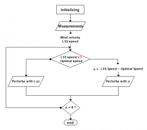
Therefore, a maximum power point tracking (MPPT) strategy is implemented to ensure an optimal functioning with an optimal power (Figure 4).
Figure 4. The adopted P&O algorithm
This algorithm can be based on a wind velocity sensor or sensorless method, with a fixed or a variable variation step [16]. One of the simplest and most used MPPT algorithms is the “Perturb and Observe” one (P&O). It consists in perturbing the low-speed shaft (LSS) velocity of the turbine, and then, observing the resulting changes in the generated power. The diagram of the implemented MPPT algorithm is given in Figure 4. It is an efficient but straightforward algorithm where the perturbation step varies according to the gap between the actual LSS speed and the desired optimal speed.
3.2.2 The HESG control loop
The HESG has strong nonlinearities. This nonlinear behavior can be noticed in Eq. (4) for instance. The electromagnetic torque Cem, expressed in the dq-frame, shows a strong coupling between the excitation current and the q-axis current.
${{C}_{em}}=p\times {{i}_{q}}\times \left[ \sqrt{3}\times \left( {{\psi }_{a}}+M{{i}_{e}} \right)\ +\ \left( {{L}_{d}}-{{L}_{q}} \right){{i}_{d}} \right]$ (4)
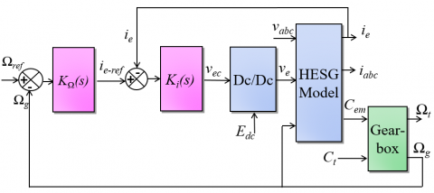
Due to the difficulty to synthesize controllers on nonlinear models, an approach involving linear control is preferred so the HESG’s model must be linearized. To take into account the errors related to linearization, a robust approach is chosen. The implemented control scheme is given in Figure 5.
The HESG’ optimal angular velocity is tracked through the adjustment of the excitation current ie to its reference. Thus, a cascaded control scheme is implemented. The control voltage vec of the DC-DC converter is generated by the inner current loop (noted Ki(s)). The excitation current reference ie-ref is generated by the external velocity loop.
The cascaded control scheme comprises an H∞ controller for the external velocity loop whereas a simple PI controller is used for the internal current loop. The robust control adopted in this work is based on the H∞ theory based on the Normalized Coprime Factors (NCF) stabilization problem [4].
The use of the NCF stabilization problem for the design of the velocity controller requires a linear model. This one is obtained through an identification of the generator-side HSS Ωg as a function of the excitation current reference ie-ref.
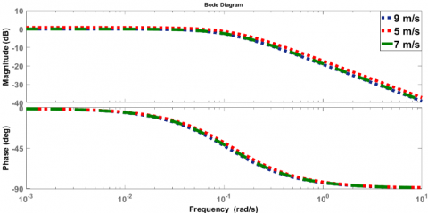
The identification procedure is performed around several operating points that cover zone II. For each operating point, a transfer function is identified, and a Bode diagram is plotted (Figure 6). An average model is then chosen. Its transfer function is given by (5). It corresponds to a wind velocity of 7 m/s. The robust controller is described in (6).
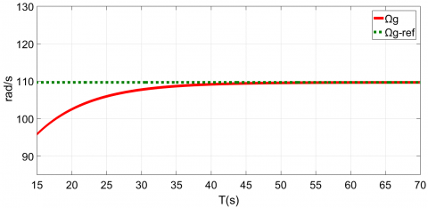
For a steady wind velocity of 7 m/s, the evolution of the angular velocity of the HESG Ωg is given in Figure 7. The velocity curve converges towards its reference.
Figure 5. The control strategy of the WCS [5]
$F(s)=\frac{\Omega_{g}}{i_{e-r e f}}=\frac{1.1}{1+8 . s}$ (5)
$K_{\Omega}(s)=\frac{0.58 s^{3}+3.91 s^{2}+0.99 s+0.06}{s^{3}+11.9 s^{2}+57.2s}$ (6)
Figure 6. Bode diagram of the identified transfer functions
Figure 7. HESG angular velocity in zone II (7 m/s)
The mechanical components include the rotor, the blades, the tower, the gearbox and both low speed and high-speed shafts.
4.1 Modeling
The modeling of the mechanical parts of the WCS must take into account the different aerodynamic aspects as well as the deflection and shear forces experienced by the structure. Such a task can be time-consuming and requires an in-depth knowledge of the wind turbine aerodynamics. Fortunately, this task can be achieved using software solutions.
In this work, the Simulink model of the HESG and the implemented power electronics are interfaced with the aerodynamic model of a wind turbine built in the CAE tool FAST.
4.1.1 FAST overview
The FAST (Fatigue, Aerodynamics, Structure, Turbulence) code is a comprehensive aeroelastic simulator capable of predicting both, extreme loads and fatigue loads of three-bladed horizontal axis wind turbines. FAST is based on advanced engineering models derived from fundamental laws such as the blade element theory and the momentum theory [17]. The combination of these two theories results in what is known as the Blade Element Momentum Theory (BEMT) used to compute the forces experienced by the wind turbine, the blades, the tour… [18]. FAST can also deliver the velocity of the rotor.
Dynamic equations derived from this theory for both kinetics and kinematics of the wind turbine are then reformulated using the Kane’s method [19] into a simplified set of motion equations solvable via numerical integration. Afterward, FORTRAN (a programming language for scientific computing invented by IBM) is used to code these equations.
FAST has its limitations. For instance, not all motions occurring during the operation of the wind turbine are taken into account [17, 20]. Moreover, in FAST, some of the models, such as the blades and the tower ones, are approximation-based models and with approximations, there is always a margin of error.
However, the considered CAE tool is very relevant for the modeling of wind turbines. It has been used in several works for different applications as described in section 1 [8, 10]. Indeed, it has also been evaluated and certified by the worldwide technical supervisory organization Germanischer Lloyd Wind Energy (currently DNV-GL). It was found suitable for the calculation of both onshore and offshore wind turbine mechanical loads for design and certification [21].
Furthermore, one of its attractiveness resides in its interfacing capabilities with Simulink or LabView. These particular features introduce more flexibility for the control implementation and the load calculations during simulation while using the full nonlinear aeroelastic wind turbine aerodynamic equations. The interfacing procedure between FAST and Simulink is given in Figure 8.
The FAST-HAWT model receives as inputs the electromagnetic torque Cem, the power Ptgenerated by the HESG as well as the control set-point for the pitch actuator βref.
The FAST code is based on several subroutines, which ensure the interaction between the aerogenerator model and the functionalities offered by the calculation tool Aerodyn [22]. By exploiting these functionalities, it is possible to retrieve several parameters such as inertias, torques and the mechanical stresses as well.
In this work, only the necessary parameters for the interfacing between FAST and Simulink are retrieved (LSS speed Ωt, pitch angle β, wind velocity, shear forces, deflection, torque, power…).
The configuration of the wind turbine as well as the simulation conditions that include the activated degrees of freedom (DOF), wind profile, generator torque, nacelle yaw, and pitch control... are chosen in the FAST’s Primary Files.
Figure 8. FAST-Simulink interfacing chart
Six degrees of freedom (DOF) are activated among the 24 available for three-bladed wind turbines, namely the vibrations in the transmission system (1DOF), the variable speed operating mode of the HSS on the generator side (1 DOF) and tower deflections in different wind directions (4 DOFs). Further characteristics of the considered wind turbine “the WindPact Baseline 1.5 MW” are given in Table 1 [23].
Table 1. Characteristics of the considered HAWT
|
Parameter |
Value |
|
Rated Power (kW) |
1500 |
|
Rotor Diameter (m) |
70 |
|
Rated LSS speed (rpm) |
20.5 |
|
Gearbox ratio (-) |
88 |
|
Cut-out wind velocity (m/s) |
27.6 |
In this section, the control of the aerogenerator in the third operating region (zone III) is described where two pitch controllers are implemented and tested.
The aerodynamic power captured by a wind conversion system (WCS) is given by (7):
${{P}_{t}}=\frac{1}{2}\ {{C}_{p}}\ \rho \ \pi \ {{R}^{2}}\ {{v}^{3}}$ (7)
where, ρ is the density of air, R is the turbine rotor radius, v is the wind velocity and Cp the power coefficient.
Cp is a function of the tip speed ratio (TSR) λ and of the pitch angle $\beta$. It is proportional to the theoretical maximum efficiency of a wind turbine set at 59.6% by the German physicist Betz.
In a classical two-mass model of a wind turbine, a mathematical approximation of Cp is needed to model the behavior of the turbine.
In the absence of an exact expression, the simulation of the coupled response of the turbine always remains inaccurate. Whereas with FAST, for the considered HAWT, the accurate value of the optimal power coefficient is given and it equals to 0.5 (50% according to the Betz theory) [23].
In the third operating region (zone III) where the wind speed exceeds its nominal value, the wind turbine must operate at its constant maximum power (1.5 MW, in our case). The aim is then to limit the extracted power, and therefore, a power control scheme must be considered. A pitch angle’s control loop (Figure 9) is implemented.
Pitch controllers can be classified into different categories and amongst them: conventional PID controllers, intelligent controllers (fuzzy logic, neural networks, genetic algorithms…), robust controllers and hybrid that combine general and soft-computing-based controllers.
Figure 9. Pitch control loop
Figure 10. Bode diagram of the identified transfer functions
In this work, two techniques are carried out: a conventional PI regulator and a PI-based fuzzy logic controller (FLC-PI). The synthesis of the proposed controllers requires a linear model. The same identification procedure adopted for the velocity loop is considered.
An identification of the generated power Pt as a function of the pitch angle βref is performed around several operating points that cover zone III. For each operating point, a transfer function is identified and a Bode diagram is plotted (Figure 10).
An average linear model is then selected to synthesize the intended regulator. Its transfer function, corresponding to an operating wind of 12 m/s, is given by (8).
$H(s)=\frac{4,9\times {{10}^{5}}}{{{{s}^{2}}}/{38,4}\;+s\times 0.12+1}$ (8)
4.2.1 PI regulation
The PI pitch regulator described in (9) receives as input, the difference between the WCS’ rated power of 1.5 MW and the power extracted from the wind (see Figure 9). As output, it generates the pitch angle reference for the three blades. The integral action of the parallel PI controller and its static gain are tuned to ensure the stability and a good reference tracking of the closed-loop.
$C(s)={{K}_{p}}+\frac{{{K}_{i}}}{s},\quad {{K}_{p}}=2.6\ \text{and}\ {{K}_{i}}=1$ (9)
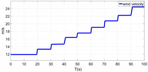
The regulator acts on the pitch actuator. It is tested for a ramp-shaped variable and uniform wind profile in the third operating region (Figure 11).
Figure 11. The considered wind profile (zone III)
Figure 12. The HESG velocity with conventional PI control
Figure 13. The Generated power in zone III (conventional PI control)
The simulated angular velocity Ωg of the HESG is given in Figure 12, it shows a satisfying shape around the lowest operating point in zone III (12 m/s), but it also reveals minor fluctuations as the wind velocity approaches its cut-out value.
As for the generated power (noted Pt), the simulation results given in Figure 13 show fluctuations. The extracted power oscillates around its rated value with an average error margin of ±1.7% around the lowest operating point in zone III (12 m/s) and ±2.8% at the highest operating point (24 m/s).
4.2.2 FLC-PI regulation
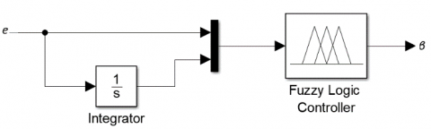
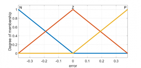
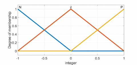
The FLC-PI designed for this application has two inputs that are the error e between the rated power and the generated one, and its integral i and only one output that is the pitch angle β. The FLC-PI architecture is given in Figure 14.
The fuzzy logic controller functioning cycle can be described as a 3-steps procedure: fuzzification, fuzzy inference and defuzzification [24]. The fuzzification consists in converting a set of crisp (real number) into a fuzzy set of values. Afterward, an inference is carried out according to a user-defined rule base. As for the defuzzification, it consists in converting the fuzzy values generated by the inference into real numbers according to user-defined membership functions.
In this work, a Sugeno-type inference is used to get more flexibility in the system design [25]. The rule base is described in Table 2, and the membership functions are given in Figure 15 and Figure 16.
Figure 14. The FLC- PI pitch controller’s architecture
Table 2. Fuzzy controller’s rules
|
i ↓ vs e → |
N |
Z |
P |
|
N |
LN |
SN |
ZERO |
|
Z |
SN |
ZERO |
SP |
|
P |
ZERO |
SP |
LP |
Figure 15. Membership function for the input “e”
Figure 16. Membership function for the input “i”
Table 3. Membership function for the output “β”
|
LN |
SN |
ZERO |
SP |
LP |
|
-5 |
-2.5 |
0 |
2.5 |
5 |
As for the output, with a Sugeno-type inference, the membership function of output β is linear. The values given in Table 3 are based on the relative movement of the pitch actuator in an amount proportional to the size of the error e.
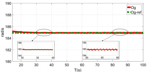
The simulation was carried out with the same wind profile used for the PI regulator (Figure 11). The simulated angular velocity of the HESG is given in Figure 17, it shows a satisfying shape around the lowest operating point in zone III (12 m/s). As the wind velocity approaches its cut-out value, the minor fluctuations observed with the conventional PI almost disappear with the FLC-PI.
Figure 17. The HESG velocity with FLC-PI control
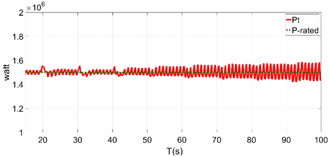
Figure 18. The generated power in with FLC-PI control (zone III)
As for the generated power (noted Pt), the simulation results (Figure 18) also show fluctuations. The extracted power oscillates around its rated value with an average error margin of ±0.8% (±1.7% with the conventional PI).
4.2.3 Investigation of the two controllers
For a ramp-shaped variable wind. As explained is section 1, hybrid excitation synchronous generators are strongly nonlinear machines mainly due to the coupling between the torque and the excitation current (6).
Besides, it is worth mentioning that the considered HESG was originally designed for electrical and hybrid traction applications and not for a use as a generator. This results in a high rate of harmonics [26]. All these reasons gathered to vibrations in the transmission system (High-Speed Shaft (HSS) – Gearbox – Low-Speed Shaft (LSS)) lead to the LSS torque ripple.
Results obtained with the two controllers, for the wind profile given in Figure 11, showed power fluctuations.
Now, considering the simple relation between the LSS torque CLSS, the gearbox ratio RGB the generated power P and the angular velocity Ωg of the HESG, given by (10), one can conclude that these power fluctuations are mainly due to the LSS torque given in Figure 19.
$P={{\Omega }_{g}}\times {{C}_{LSS}}\times {{R}_{GB}}$ (10)
The results confirm that the FLC-PI controller minimized the fluctuations of the angular velocity (see Figure 17 compared to Figure 12) and thus, the vibrations in the transmission system.
Consequently, the torque ripple is also minimized. This conclusion about the FLC-PI performances is confirmed in Figure 20.
Figure 19. The LSS torque with both controllers
Figure 20. The generated power with both controllers
The electromagnetic torque ripple is mainly due to the vibrations in the transmission system, as well as to the shear forces experienced by the flexible blades, the tower, and the drive shaft. The mentioned loads confirm the capabilities of the developed model as a tool to simulate the realistic aerodynamic behavior of the considered WCS. This was not possible with a classic mechanical model such as a two-mass model for example. Figure 21 shows a 30 seconds simulation of the blades pitch position obtained with both proposed controllers.
All calculations are made under a wake induction model based on the BEMT theory and optimal airfoils. These loads can be used to calculate local stresses using a cross-sectional analysis. The difference between the two pitch controllers is clear in Figure 21. The negative values reflect the aerodynamic twist of the blades.
As information, the optimal pitch is near zero degrees. With such an aerodynamic twist, the minimum blade-pitch angle tends to be saturated [27].
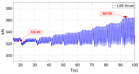
The bending moment applied by the edge of the blade on the hub is given in Figure 22 and the thrust forces experienced by the rotor-side low-speed shaft are given in Figure 23.
The turbine rotor design study carried out by Malcolm and Hansen [23] for the considered HAWT (WindPact 1.5 MW Baseline) shows a maximum blade root edgewise moment of 815 kN.m and a maximum LSS thrust of 324 kN.m.
In this study, the loads were simulated with the standard International Electro technical Commission (IEC) Kaimal spectrum [28] for an optimum operation in turbulence.
Regarding the different operating conditions, such as the wind profile and the activated DOFs, Figure 22 and Figure 23 show a good agreement with the results given by Malcolm and Hansen [23] around the lowest operating point in zone III but more severe loads around the cut-out wind velocity.
Figure 21. Blade 1 pitch position
Figure 22. Blade 1 edgewise moment
Figure 23. Thrust experienced by the LSS
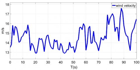
For a stochastic wind in zone III. For more severe simulation conditions under a turbulent wind resulting in much important loads, especially on the blades, the two controllers are also tested for a stochastic wind profile in the third operating region (Figure 24).
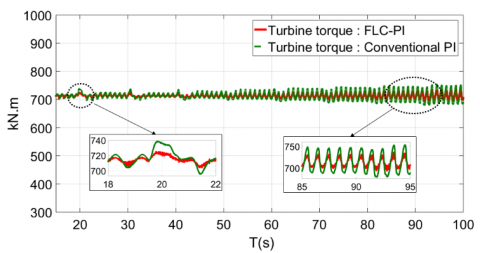
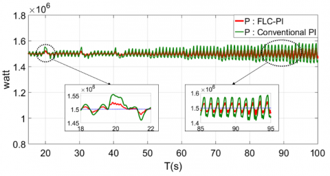
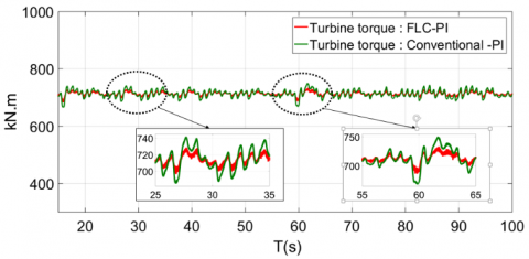
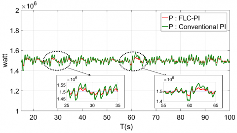
The LSS torque and the generated power obtained with both controllers for this particular wind profile are given in Figure 25 and Figure 26, respectively.
Figure 24. Considered stochastic wind profile in zone III
Figure 25. LSS torque with both controllers
Figure 26. Generated power with both controllers
The LSS torque ripple is reduced with the PI-based fuzzy logic controller as well as the fluctuations in the generated power with an average value of 50 kW.
The obtained results confirm the better performances of the FLC-PI compared to the conventional PI controller. It also shows a good shape under the considered wind profile.
In this paper, an advanced aerodynamic model for a variable speed HESG-based WCS is proposed. The CAE tool FAST is used to interface an electromagnetic model that considers complex electrical phenomena, especially space harmonics generated by the HESG and time harmonics caused by the converters switching effects, with an aerodynamic HAWT’s model.
As for the control strategy, a robust H∞ controller is considered for the HESG velocity loop and two pitch control techniques are tested and investigated.
The simulation results reflect the model’s capabilities for further studies such as structural analysis and performances' evaluation. It also demonstrates the superior capabilities of soft-computing-based controllers compared to conventional ones for the pitch control of a 1.5 MW variable speed wind turbine. The FLC-PI is found to be more adequate; it has shown better time responses and a better accuracy especially for the ramped-shaped wind profile.
The thrust at the low-speed shaft (LSS) and the blades root edgewise moment are given. The simulation has shown a good agreement with previous loads analysis studies around the rated wind velocity. However, these fatigue-related forces are still significant as the wind velocity approaches its maximum value and further investigations should be conducted to reduce its effect on the structure of the wind turbine.
More efficient control techniques will be investigated. Grid connection is already an ongoing subject, torque ripple minimization will be considered and the optimization of the topology of the considered HESG is under study.
|
BEMT |
blade element momentum theory |
|
|
CAE |
computer-aided engineering tool |
|
|
Cem |
electromagnetic torque of the HESG, N. m |
|
|
CLSS |
low-speed shaft torque, N. m |
|
|
Cp |
power coefficient of the wind turbine |
|
|
DOF |
degree of freedom of the wind conversion system |
|
|
e |
error between the generated and the rated power of the wind turbine |
|
|
FLC |
fuzzy-logic controller |
|
|
HAWT |
horizontal-axis wind turbines |
|
|
HESG |
hybrid excitation synchronous generator |
|
|
HSS |
high-speed shaft of the wind turbine |
|
|
i |
integral of the error |
|
|
ie |
excitation current of the HESG, A |
|
|
ie-ref |
excitation current reference generated by the inner current loop, A |
|
|
Ki |
integral gain of the PI pitch controller |
|
|
Kp |
proportional gain of the PI pitch controller |
|
|
L |
self-inductance of the HESG |
|
|
LLS |
low-speed shaft of the wind turbine |
|
|
Ls0 |
continuous component of the self-inductance of the HESG |
|
|
M |
mutual inductance of the HESG |
|
|
Ms0 |
continuous component of the mutual inductance |
|
|
POR |
fictive point of regulation |
|
|
Pt |
total power generated by the WCS, W |
|
|
RGB |
gearbox ratio |
|
|
vec |
control voltage generated by the DC-DC converter, V |
|
|
WCS |
wind conversion system |
|
|
Greek symbols
|
|
|
|
β |
actual pitch angle of the blades, rad |
|
|
βref |
pitch angle reference generated by the pitch controller, rad |
|
|
Ɵ |
Angular position of the HESG’s rotor, rad |
|
|
λ |
tip speed ratio of the wind turbine |
|
|
ρ |
air density, kg. m-3 |
|
|
ϕe |
total flux created in the airgap, Wb |
|
|
Ωg |
angular velocity of the HESG, rad. s-1 |
|
|
Ωt |
angular velocity of the low-speed shaft |
|
[1] Global Statistics. (2017). Global Wind Energy Council. www.gwec.net.
[2] Global review. Renewable Energy Policy Network for the 21st Century. (2017). www.rne21.net.
[3] Vido, L., Gabsi, M., Lecrivain, M., Amara, Y., Chabot, F. (2005). Homopolar and bipolar hybrid excitation synchronous machines. IEEE International Conference on Electric Machines and Drives, pp. 1212-1218. https://doi.org/10.1109/IEMDC.2005.195876
[4] Berkoune, K., Ben Sedrine, E., Vido, L., Le Ballois, S. (2014). Robust Control of Hybrid Excitation Synchronous Generator for Wind Applications. Mathematics and Computers in Simulation, Elsevier (MatCom), 131: 55-75. https://doi.org/10.1016/j.matcom.2015.10.002
[5] Mseddi, A., Le Ballois, S., Vido, L., Aloui, H. (2016). An integrated Matlab-Simulink platform for a wind energy conversion system based on a hybrid excitation synchronous generator. 11th International Conference on Ecological Vehicles and Renewable Energies, Monaco. https://doi.org/10.1109/EVER.2016.7476357
[6] Ramtharan, G., Jenkins, N., Anaya-Lara, O., Bossanyi, E. (2007). Influence of rotor structural dynamics representations on the electrical transient performance of FSIG and DFIG wind turbines. Wind Energy: An International Journal for Progress and Applications in Wind Power Conversion Technology, 10(4): 293-301. https://doi.org/10.1002/we.221
[7] Boukhezzar, B., Siguerdidjane, H. (2011). Nonlinear control of a variable-speed wind turbine using a two-mass model. IEEE Transactions on Energy Conversion, 26(1): 149-162. https://doi.org/10.1109/TEC.2010.2090155
[8] Benbouzid, M., Beltran, B., Mangel, H., Mamoune, A. (2012). A high-order sliding mode observer for sensorless control of DFIG-based wind turbines. IECON 2012-38th Annual Conference on IEEE Industrial Electronics Society, pp. 4288-429. https://doi.org/10.1109/IECON.2012.6389200
[9] National Renewable Energy Laboratory. FAST CAE tool. (2018). https://nwtc.nrel.gov/FAST.
[10] Hayat, K., Asif, M., Ali, H.T., Ijaz, H., Mustafa, G. (2015). Fatigue life estimation of large-scale composite wind turbine blades. 12th International Bhurban Conference on Applied Sciences and Technology (IBCAST), pp. 60–66. https://doi.org/10.1109/IBCAST.2015.7058480
[11] Gardner, P., Garrad, A., Hansen, L.F., Tindal, A., Cruz, J.I., Arribas, L., Fichaux, N. (2009). Wind energy-The Facts Part 1 Technology. European Wind Energy Association (EWAE).
[12] Hansenm M.O.L. (2015). Aerodynamics of Wind Turbines. Routledge, Taylor and Francis Group.
[13] Cognet, V., Courrech du Pont, S., Dobrev, I., Massouh, F., Thiria, B. (2017). Bioinspired turbine blades offer new perspectives for wind energy. Proceedings of the Royal Society A: Mathematical, Physical and Engineering Sciences, 473(2198): 20160726. https://doi.org/10.1098/rspa.2016.0726
[14] Hoogedoorn, E., Jacobs, G. B., Beyene, A. (2010). Aero-elastic behavior of a flexible blade for wind turbine application: A 2D computational study. Energy, 35(2): 778-785. https://doi.org/10.1016/j.energy.2009.08.030
[15] Vido, L. (2004). Étude d’actionneurs électriques à double excitation destinés au transport : Dimensionnement de structures synchrones. PhD thesis in Electrical Engineering, Ecole Normale Supérieure de Cachan (ENS Cachan).
[16] Abdullah, M.A., Yatim, A.H.M., Tan, C.W., Saidur, R. (2012). A review of maximum power point tracking algorithms for wind energy systems. Renewable and Sustainable Energy Reviews, 16(5): 3220-3227. https://doi.org/10.1016/j.rser.2012.02.016
[17] Wilson, R.E., Walker, S.N., Heh, P. (1999). Technical and User’s Manual for the FAST_AD Advanced Dynamics Code. OSU/NREL Report 99-01.
[18] Glauert, H. (1935). Airplane Propellers. Aerodynamic Theory. Springer, Berlin, Heidelberg, pp. 169-360.
[19] Kane T.R., Levinson D.A. (1985). Dynamics, Theory and Applications. McGraw Hill.
[20] Jonkman, J.M., Buhl Jr, M.L. (2005). FAST user’s guide. National Renewable Energy Laboratory, Technical Report No. NREL/EL-500-38230, Golden, CO, USA.
[21] Manjock A. (2005). Design codes FAST and ADAM for load calculations of onshore wind turbines. Germanischer Lloyd WindEnergie GmbH, Report No. 72042, Hamburg.
[22] Jonkman, J.M., Hayman, G.J., Jonkman, B.J., Damiani, R.R. (2015). AeroDyn v15 User’s Guide and Theory Manual. NREL Draft Report, Golden, CO, USA.
[23] Malcolm D.J., Hansen A.C. (2006). WindPACT Turbine Rotor Design Study: June 2000--June 2002 (Revised). National Renewable Energy Lab. (NREL), Golden, CO, USA. https://doi.org/10.2172/15000964
[24] Bai, Y., Wang D. (2006). Fundamentals of fuzzy logic control — fuzzy sets, fuzzy rules and defuzzifications. In: Bai Y., Zhuang H., Wang D. (eds) Advanced Fuzzy Logic Technologies in Industrial Applications. Advances in Industrial Control. Springer, London. https://doi.org/10.1007/978-1-84628-469-4_2
[25] Sabri N., Aljunid S.A., Salim M.S., Badlishah R.B., Kamaruddin, R., Malek M.A. (2013). Fuzzy inference system: Short review and design. International Review of Automatic Control, 6(4): 441-449.
[26] Mseddi, A., Le Ballois, S., Aloui, H., Vido, L. (2018). Investigation of two torque ripple minimization techniques of a HESG in a wind conversion. 2018 XIII International Conference on Electrical Machines (ICEM), pp. 2192-2197. https://doi.org/10.1109/ICELMACH.2018.8507263
[27] Jonkman J.M. (2018). NREL's National Wind Technology Center Forum. https://wind.nrel.gov/forum/wind.
[28] International Electrotechnical Commission. (1998). Safety of Wind Turbine Conversion Systems. 61400-1. Chicago. IL: International Electrotechnical Commission.