Caroline Stackler* | Florent Morel | Philippe Ladoux | Piotr Dworakowski
© 2020 IIETA. This article is published by IIETA and is licensed under the CC BY 4.0 license (http://creativecommons.org/licenses/by/4.0/).
OPEN ACCESS
This paper presents a methodology for the modelling of a 25 kV-50 Hz railway infrastructure, for frequencies from 0 to 5 kHz. It aims to quantify the amplifications of current and voltage harmonics generated by on-board converters into the infrastructure. A circuit is developed to model the skin effect in the overhead line for time-domain simulations. A new approach, based on state space representation and transfer functions, is also proposed to analyze the interactions between trains. The methodology is then applied in Matlab-Simulink and validated with EMTP-RV. Harmonic interactions between the infrastructure and on-board converters are analyzed. Then, an extension of the model is proposed for higher frequencies in order to study harmonic interactions between new on-board converters and the infrastructure.
railway supply, impedance, skin effect, state space representation, harmonic interactions, EMC
Nowadays, different architectures of on-board converters coexist in the railway infrastructure [1]. Current topologies are generally composed of an input step-down multiwinding transformer supplying input active rectifiers [1]. New topologies, including medium frequency transformers, are currently studied to replace the on-board AC-DC conversion stages, as presented in the researches [2-5]. Thanks to the development of these new structures, a diminution of on-board weight and volume, an increase of the availability and an improvement of the efficiency are expected [6].
In any cases, the on-board converters use semiconductor switches which generate harmonics at the pantograph level. They are then injected into the infrastructure and they interact with the impedance of the railway line. If amplified, they can cause disturbances in the overhead line voltage and may disrupt rail signalling or other trains running on the same sector [7]. Thus, the harmonic level tolerated in the overhead line is limited by interoperability standards and constraints imposed by railway companies. As an example, the maximum peak voltage at every point of the infrastructure cannot exceed 50 kV to comply with the European standard EN 50388 [8]. In addition, at some frequencies dedicated to signalling, no harmonic is allowed.
In order to analyse the impact of disturbances on the network and to ensure the compliance with standards, a model of the railway infrastructure has to be developed for the frequency range of the harmonics generated by the on-board converters.
After a short state of the art on the classical methodology of 25 kV-50 Hz railway infrastructure modelling for frequencies up to 5 kHz, some innovative approaches are proposed. First, a circuit for overhead line skin effect modelling in the time domain is presented. A state-space representation based approach is also developed. Studies with several trains running on the same sector and the analysis of the impact of one train on another are hence simplified. These models are illustrated by simulations performed in the environment Matlab-Simulink. Then, the Simulink models are compared with models implemented in EMTP-RV. The harmonic interactions between the 25 kV-50 Hz railway infrastructure and on-board multilevel converters controlled by phase shifted pulse width modulation are also analysed. Finally, the infrastructure models are extended for frequencies up to a few tens of kilo hertz in order to prepare the new on‑board multilevel converters for certification.
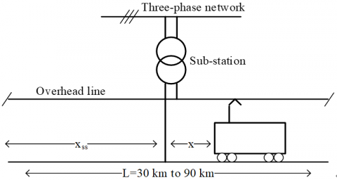
A 25 kV-50 Hz railway infrastructure is generally constituted of electrically independent sectors from 30 to 90 km (Figure 1 [1]). Every sector is supplied from the three-phase grid thanks to a substation single phase transformer, connected between two phases of the grid.
A single phase railway infrastructure can then be modelled by a 30 to 90 km line sector supplied with the substation transformer. The three phase network and the substation transformer may be roughly modelled by lumped series inductances and resistances [1]. However, comparing the wave length at 5 kHz in the overhead line (59 km) to the sector length, one can notice that the propagation effects cannot be neglected. Thus, distributed parameters should be used instead of lumped parameters to model the overhead line. Generally, the theory of multi-conductor transmission lines (MTL) and the telegrapher's equations are used to describe the overhead line and the rails, taking into account the propagation effects [1, 7, 9-11]. Up to 5 kHz, it has been shown by Ferrari et al. in 1998 [9] that the overhead wires can be reduced to a single equivalent conductor model, assuming the contact and catenary wires connected in parallel. Beyond 5 kHz, interactions between overhead wires, soil conductivity and rail geometry impact, a priori, this assumption.
Figure 1. Diagram of a 25 kV-50 Hz infrastructure sector
The telegrapher's equations use hyperbolic sines and cosines of complex variables. Thus, in order to simplify the implementation of the telegrapher's equations in some software specialized in time domain simulations, the line can be discretized in quadripoles associated in cascade.
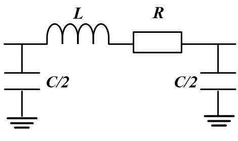
The quadripoles are composed of lumped parameters. Their length has to be small compared with the minimum wave length considered to neglect the propagation effects and to use lumped parameters instead of distributed parameters. Thus, it depends on the frequency range. Figure 2 and Figure 3 present the model of an infinitesimal section of the single-conductor equivalent line with distributed parameters and the model of a quadripole.
The impedance seen by the train has been analytically calculated on the reduced model. The quadripole association has also been implemented in Matlab-Simulink, using the toolbox SimPowerSystems. Both calculation methods have been applied on an infrastructure sector. The parameters were calculated thanks to the tool "power_lineparam" from the SimPowerSystems library in Matlab [12] and the data [1]. They are given in Table 1. The different lengths correspond to the ones given in Figure 1. The quadripoles in the discretized model are 1 km long to be short enough compared to the wave length at 5 kHz, equal to 59 km.
Figure 4 presents the impedance seen by the train for both models (telegrapher's equations and cascaded quadripoles). One can see that the results coincide exactly. Thus, the discretization with 1 km long quadripoles is a fair approximation of the multiconductor transmission line theory for this frequency range.
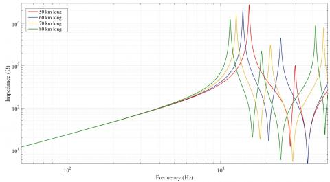
Then, a study has been made to quantify the impact of the infrastructure geometry and the train position on the impedance. To do this, the impedance seen by the train has been calculated for different line sectors and different train positions. Figure 5 shows the results for a train on some different sectors. The substation is in the middle of the sector and the train at 10 km from the sub-station. The per-unit-length parameters and the substation parameters are given in Table 1.
One can notice resonances in the impedance at some characteristic frequencies. If harmonics are generated by an on-board converter running on the sector at one of these resonant frequencies, they would be highly amplified by the infrastructure. Thus, an overvoltage could be caused in the overhead line. One can also see that the resonant frequencies depend on the sector on which the train runs. It has also been shown that these resonances depend on the train position [13, 14].
Figure 2. Equivalent circuit of a single equivalent conductor overhead line
Figure 3. Equivalent circuit of an overhead line quadripole with lumped parameters
Table 1. Parameters of the sector
|
Overhead line per-unit-length parameters |
$r=0.16 \Omega / \mathrm{km}$ |
$l=1.6 \mathrm{mH} / \mathrm{km}$ |
|
Sub-station parameters |
$R_{s s}=1.17 \Omega$ |
$L_{\mathrm{fi}}=21.2 \mathrm{mH}$ |
|
Lengths |
$L=50 \mathrm{km}$ |
$x_{s s}=20 \mathrm{km}$ |
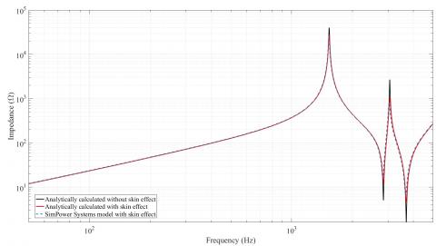
From a few hundreds hertz, the skin depth becomes smaller than the line radius, typically 5.8 mm for a catenary in copper. Thus, the skin effect impacts the overhead line resistance. In order to quantify its impact on the impedance of the infrastructure, a comparison has been made. It is shown in Figure 6, between analytical calculations of the impedance seen by a train running on the sector without and with skin effect. The studied infrastructure sector is the one presented in the previous section with the parameters given in Table 1.
One can notice that the skin effect has a significant impact on the resonances. Indeed, it tends to attenuate their amplitude. Besides, with the increasing frequency, this attenuation becomes more significant. For example, in Figure 6, the impedance at 2.5 kHz, the second resonance, is divided by three between the model without skin effect and the one with skin effect.
However, one can see that the skin effect does not impact the resonant frequencies. Thus, neglecting the skin effect overestimates the amplitude of the resonances.
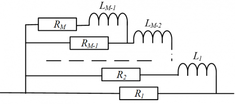
In order to model the frequency dependence of the line resistance in a time domain simulation software, a ladder circuit composed of resistances and inductances, as shown in Figure 7, has been studied for transmission lines by Sen and Wheeler [15], and Yen et al. [16]. The resistances and inductances are chosen with, respectively, decreasing and increasing values. At low frequency, the circuit is equivalent to the resistances associated in parallel. When the frequency increases, the contributions of the inductances increase. The impedance of the external branches $R_{i}+j \omega L_{i-1}$ becomes high in front of $R_{i-1}$ and the association in parallel of $R_{i-1}$ and $R_{i}+j \omega L_{i-1}$ can be approximated by $R_{i-1}$. Thus, the impedance of the circuit increases from the association in parallel of all the resistances to the resistance $R_{1}$, when the frequency increases.
The values of resistances and inductances are calculated by an optimisation algorithm with the objective of minimizing the error (1) between the real part of the ladder circuit ($\operatorname{Re}\left(Z_{R L}(f)\right)$) and the resistance with skin effect of a line quadripole analytically calculated ($R_{A C}(f)$) in the considered frequency range [17].
Figure 7. Equivalent ladder circuit modelling the skin effect in transmission lines
error$=\sum_{f=f_{0}}^{f_{\max }}\left(\frac{\operatorname{Re}\left(Z_{R L}(f)\right)-R_{A C}(f)}{R_{A C}(f)}\right)^{2}$ (1)
Some constraints are imposed to ensure an accurate model at the fundamental frequency and a small imaginary part compared to the inductance of a quadripole.
To reach convergence, the initial parameters have to be well-chosen. Thus, the optimisation is realised in several steps by increasing the number of levels in the ladder circuit. Each iteration takes as initial parameters the result of the previous iteration. The algorithm of the optimisation is shown in Figure 8 and it is developed by Stackler et al. [14].
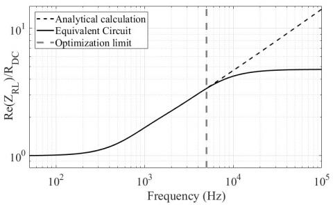
A 3-resistance 2-inductance ladder circuit has been obtained, both complying with the constraints and fitting with the resistance with skin effect up to 5 kHz. However, more resistances and inductances are necessary to have a fair model at higher frequencies. The real part of the result of the optimization is compared to the quadripole resistance with skin effect on Figure 9.
Replacing the resistances in the line quadripoles by the obtained RL ladder circuit, the skin effect can quite easily be taken into account in the time domain simulation. A model using the cascaded quadripole theory presented in section 2 and the RL ladder circuit modelling the skin effect has been realised in Matlab-Simulink, using the toolbox SimPowerSystems.
In this model, one quadripole models 1 km of the overhead line. The resulting impedance seen by a train on the sector is drawn in blue in Figure 6, validating the model up to 5 kHz. An illustration of this model is shown Figure 10.
Figure 8. Flowchart of the optimisation algorithm
Figure 9. Comparison between the normalized real part of the optimized ladder circuit and the analytical calculation of the resistance with skin effect for a 3-level ladder circuit
Figure 10. Railway infrastructure modelled by cascaded quadripoles including RL ladder circuit for skin effect modelling
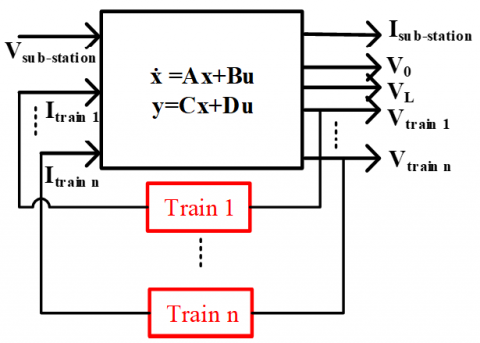
In order to simplify the consideration of several trains running on the same railway sector, a new approach, based on the state-space representation of the infrastructure has been developed. It is illustrated in Figure 11.
The state-space representation of the railway infrastructure is calculated with, at input, the substation transformer voltage, $V_{\text {sub}-\text {station}}$ and the currents in the trains' pantographs $I_{\text {trains}}$. The outputs are the currents and voltages at different points of the line, such as the substation current of the voltages at the trains' terminals or at the extremities of the line. The states of such a representation correspond to the voltages at the terminals of the capacitors and the currents in the inductances of the line quadripoles. With a model of the trains, simulations with several trains running on the same infrastructure sector can easily be made.
Figure 11. State-space diagram of the traction chain and the infrastructure
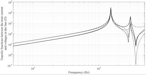
Typically, the state space representation of a railway infrastructure modelled by 1 km long quadripoles associated in cascade in which each resistance is modelled by a 5‑resistance 4-inductance circuit, counts hundreds of states. Thanks to Matlab-Simulink, the state space representation of the infrastructure can be automatically computed. Then, the transfer functions between every input and output can be easily determined from the state space representation. Hence, the influence of a specific input on an output can be analysed. Figure 12 presents some examples of transfer functions from a train current to voltages in the overhead line. Thanks to these transfer functions, the voltage harmonics caused by the amplification of current harmonics generated by a train on the sector can be estimated. For example, in Figure 12, the highest impedance value at 3 kHz is six times higher than the lowest value. Thus, current harmonics generated at 3 kHz. by on-board converters would be more or less amplified depending on the position of the train on the line.
Figure 12. Examples of transfer functions between a train current and voltages in different points of the line
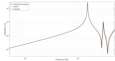
Figure 13. Comparison of impedances seen by a train on the sector according to the used method or software
Direct measurements on real lines are most of the time impossible. Indeed, both the installation for impedance measurements with a wide frequency range and the access to railway infrastructures are quite limited.
In order to validate the approaches based on analytical calculations and SimPowerSystems modelling, a study has thus been carried out in EMTP-RV (ElectroMagnetic Transient Program) [18], a software specialized in power system studies and transients analysis.
To validate Matlab-Simulink models, the infrastructure sector studied previously has been modelled in EMTP-RV using a frequency-dependent line model proposed by the software. The line parameters are calculated from the geometrical and physical parameters of the sector given in Table 2 and used to calculate the parameters used in Matlab-Simulink model.
Table 2. Parameters of the sector for EMTP-RV modelling
|
DC resistance |
$0.16 \Omega / \mathrm{km}$ |
|
Line radius |
$5.8 \mathrm{mm}$ |
|
Vertical height |
$5.5 \mathrm{m}$ |
|
Soil resistivity |
$0 \Omega \mathrm{m}$ |
|
Number of conductors |
1 |
One can notice that the impedance seen by the train obtained with EMTP-RV model coincides with both analytical calculation and SimPowerSystems model for frequencies up to 5 kHz. Thus, the frequency behaviour of Matlab-Simulink model is validated.
The harmonic interactions between an on-board converter and the railway infrastructure have then been analysed for two different sectors.
6.1 Input on-board converter
Most of the modern on-board converters running on AC railway infrastructures are constituted by a low frequency multiwinding transformer at input which steps down the supply voltage from the infrastructure. On the transformer secondaries, there are connected active rectifiers generating DC voltages to supply the three-phase inverters which control the AC traction motors. The principle diagram of these converters is presented on Figure 14.
The new on-board multilevel converter topologies including medium frequency transformers are currently studied to reduce the on-board weight and volume and increase the efficiency of the traction chain [2-6, 19]. These converters are composed of several identical physical levels or cells associated in series at input and connected in parallel at output on the DC bus supplying traction motors through three‑phase inverters. Each physical level is constituted by an AC-DC converter supplying a floating DC bus on which is connected an isolated DC-DC converter including a medium frequency transformer. The diagram of this topology is shown in Figure 15.
Figure 14. On-board converter with a low frequency transformer (only one rectifier is drawn)
Figure 15. Power Electronic Transformer (PET)
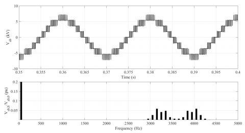
In both topologies, the input AC-DC conversion stage is controlled with interleaved pulse width modulation. Thus, the voltage at the train terminal can be seen as the sum of the voltage in either the leakage inductance of the input transformer or the input inductance of the converter and a multilevel voltage presenting 2N+1 steps, where N is, respectively for both topologies, the number of active rectifiers or physical levels [20]. This typical voltage and the corresponding spectrum are shown in Figure 16 [21].
Thanks to the pulse width modulation, low order harmonics are cancelled. However, high frequency harmonics, centred on multiples of twice the switching frequency, are generated. Shifting the carriers used to control every physical level by the same angle $\frac{\pi}{N}$, the harmonics are rejected at higher frequencies and thus, the total harmonic distortion is reduced [21]. For an association of N full bridges, the apparent switching frequency on which are centred the harmonics, is defined as the switching frequency multiplied by the number of H-bridges $N f_{s w}$. For example, for a 4-cell converter controlled with a switching frequency of 450 Hz, the first harmonic block is centred at 3.6 kHz, as shown in Figure 16.
The on-board converters are modelled in Matlab-Simulink. The skin, proximity and capacitive effects are neglected in the models of the input step down transformer. They should, a priori, have an impact on the harmonic amplitudes.
6.2 Harmonic interactions
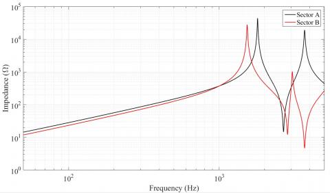
Two different sectors have been modelled in Matlab-Simulink. Both sectors have the same per-unit-length and substation parameters, which are given in Table 1. Sector A is 40 km long, with a sub-station in the middle and a train running at 5 km from one extremity of the line. Sector B corresponds to the sector presented in section 3, Table 1. The impedances seen by a train on both sectors A and B are presented Figure 17.
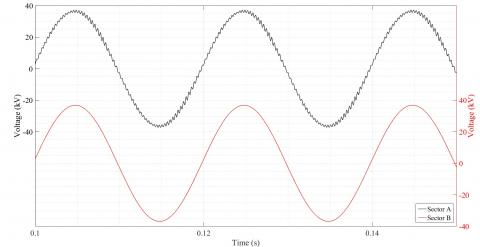
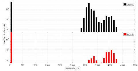
The study was carried in Matlab-Simulink with a train modelled as described previously and controlled by phase shifted pulse width modulation with a switching frequency of $f_{s w}=450 \mathrm{Hz}$. The voltages at the train terminals on both sectors A and B are drawn Figure 18 and the corresponding spectra are shown Figure 19.
One can notice, in Figure 18, some disturbances in the voltage on the sector A, whereas the voltage on the sector B seems quite sinusoidal. By analyzing the corresponding spectra presented in Figure 19, one can see that both voltages present a harmonic bloc centered around $3.6 \mathrm{kHz}$ as expected. However, the harmonics are much more amplified on the sector A. For example, the maximum voltage harmonic on the sector A corresponds to 4 % of the fundamental, to be compared with less than 0.1 % on the sector B.
By comparing the amplitudes of the impedances seen by the train on both sectors, one can see that on the sector A, the impedance seen by the train at $3.6 \mathrm{kHz}$, is equal to $5 k \Omega$ while the one on the sector B is smaller than $20 \Omega$. Thus, the amplification at $3.6 \mathrm{kHz}$ in the sector B is more than 250 times smaller than in the sector A. That is why, the harmonic bloc around $3.6 \mathrm{kHz}$ is much more amplified in the sector B than in the sector A.
Figure 16. Voltage and spectrum generated in input of the 4-cell converter with a switching frequency
Figure 17. Impedances seen by the train on both sectors A and B
Figure 18. Voltages at the train terminals on both sectors
Figure 19. Voltage frequency spectra at the train terminals on both sectors. Out of concern for visibility, the scale is logarithmic and has been maintained for both spectra. Indeed, with a linear scale, the harmonics are not visible in the voltage spectrum on the sector B using the same scale
In future on-board multilevel converters including medium frequency transformers (see Figure 15), several H-bridges have to be connected in series in input to withstand the infrastructure voltage. The number of levels depends on the voltages of the intermediate DC buses, and so, on the semiconductors used for the AC-DC conversion. Nowadays, semiconductors can withstand no more than a few kilovolts, which results in a number of rectifiers quite high. As explained in section 6, the harmonics generated by on-board converters controlled by phase shifted pulse width modulation depend on the number of cells. Higher is this number, lower is the total harmonic distortion and higher are the frequencies at which harmonics are generated. Thus, new on-board multilevel converters will, a priori, generate harmonics at frequencies higher than 5 kHz, as long as semiconductors do not withstand higher voltages. So, to study harmonic interactions between some new on-board converters and the railway infrastructure, the modelling proposed in the previous sections has to be extended up to a few tens of kilo hertz.
Nevertheless, the models cannot be directly used for higher frequency simulations because the single equivalent conductor reduction presented in section 2 is not valid beyond 5 kHz. Indeed, the interactions between wires and the soil conductivity have, a priori, an influence which makes this assumption non valid.
As it cannot easily be extended, a bibliographic study has been made in order to predict the behaviour of the infrastructure when the frequency increases. The problem is that in the literature, every railway infrastructure modelling is either made for low frequency study, thus below 5 kHz, or for high frequency study for Electromagnetic Compatibility (EMC) and thus over 100 kHz.Thus, no study has been found between 5 kHz and 100 kHz.
First, some discontinuities have been neglected. For example, the overhead line is carried by masts located every 50 to 70 m at 3 m from the track axis [22]. Moreover, the catenary is composed of different wires, at least a contact wire and a suspension wire, which are regularly connected together. It has been shown by Cozza [22] that below a few mega hertz, these discontinuities are negligible.
Two other aspects could also impact the infrastructure model: the rails and the ballast on which it lays. Generally, the image principle is used to calculate the per-unit-length parameters [1]. However, the low conductivity of the ballast impacts the capacitance between the rails and the ground. Moreover, in order to calculate the per-unit-length parameters using the image principle, the considered conductors have to be cylindrical and sufficiently far from the soil. Thus, the rail geometry and their low height impact, a priori, the calculation of the parameters. However, it has been showed in the study [22] that their impact is negligible under a few mega hertz.
Other effects, which were neglected before, are the frequency and parasitic effects in the sub-station transformer. So far, the sub-station transformer has only been modelled by a resistance and an inductance. However, other parameters, such as parasitic capacitors and magnetizing inductance, have an influence, a priori, on the impedance of the infrastructure. Moreover, when the frequency increases, both the skin and the proximity effects increase. Indeed, in the transformer, several conductors are close to each other and thus, are subject to proximity effects in addition to the skin effect in the resistance of the windings. Both these frequency effects result in an increasing of the resistance of the transformer winding with the frequency [1]. As shown both by Suarez [1] and Ouaddi et al. [23], under a few tens of kilo hertz, these phenomena result in an attenuation of the resonances in the infrastructure impedance.
It is also shown that the soil conductivity impacts the infrastructure impedance [22, 24]. First, the soil was modelled as a perfect conductor. However, its real conductivity is not infinite. Thus, the per-unit-length parameters have to be recalculated taking into account the soil conductivity, which tends to attenuate the amplitude of the resonances in the infrastructure impedance.
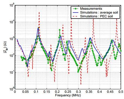
The behaviour at higher frequencies has been verified experimentally in the research [22]. An example is given in Figure 20, for a 2.75 km sector at the Centre d'Essai Ferroviaire (CEF) in Valenciennes, France. Measurements on a real line have been compared with analytical calculations based on the multiconductor transmission line theory. The per-unit-length parameters of the model have been calculated thanks to the image principle in case of a perfectly conductive soil (PEC) and of a lossy soil (average soil).
One can see that the resonances are attenuated when the conductivity of the soil is not infinite compared to a soil modelled as a perfect conductor. One can also notice that for frequencies up to a few tens of kilo hertz, the impedance obtained with the model with a lossy soil is close to the one measured on the line, validating, a priori, the modelling for this frequency range. However, it is important to notice that all the tests were carried out on a short infrastructure regarding real line sectors and thus, have to be qualified. Besides, the resonances in the line impedances are higher in frequency, and the frequency effects are more important than in real lines.
Eventually, below a few tens of kilo hertz, every aspect of the infrastructure, which was neglected below 5 kHz, seems either not to impact or to attenuate the resonances in the infrastructure impedance. As a first approximation, the modelling presented in this paper can be extended for frequencies up to a few tens of kilo hertz. A priori, the upper limit of the impedance seen by a train thus obtained, is a rough over-estimation of the real amplification of the infrastructure, which could be refined by accurate studies.
Figure 20. Comparison between measurements on a 2.75 km line and modellings with soil assumed as a perfect electrical conductor (PEC soil) and as a lossy soil (average soil) [22]
In this paper, a methodology for 25 kV-50 Hz railway infrastructure modelling has been presented. First, the 25 kV-50 Hz infrastructure and a state of the art on the railway infrastructure modelling based on the MTL theory have been presented. Then, a modelling in Matlab-Simulink environment has been proposed. It includes an equivalent circuit, composed by resistances and inductances disposed in ladder, for skin effect modelling in the overhead line resistance in the time domain. A new approach based on the state space representation of the infrastructure has also been developed. This approach makes it easier to take into account several trains running on the same catenary sector while reducing the simulation time. Thanks to the transfer functions deduced from the state space representation, it is also possible to analyse the impact of one train on another train running on the same sector.
Then, the infrastructure modelling realised in the environment Matlab-Simulink has been validated thanks to simulations in EMTP-RV, dedicated to transient analysis and line modelling.
By analysing the impedance seen by a train running on the infrastructure, some resonances at characteristic frequencies have been highlighted. Comparing the modelling without and with skin effect, it has been shown that the skin effect in the line resistance attenuates the amplitudes of the resonances of the infrastructure impedance. It has then been exposed that the resonant frequencies of the infrastructure impedance are dependent on the sector geometry and the train position. For this reason, boundaries were computed for further worst-case analysis.
Then, this model has been used to study the harmonic interactions between an on-board converter and the infrastructure. In particular, the amplifications, in the infrastructure, of the harmonics generated by the on-board converter have been analysed in function of the sector geometry.
Thanks to a bibliographic study, the infrastructure model has then been extended to frequencies up to a few tens of kilo hertz in order to study the harmonic interactions between new on-board converters and the railway infrastructure.
The infrastructure modelling methodology presented in this paper takes into account some frequency dependent phenomena such as the propagation and the skin effect in the overhead line. Nevertheless, this modelling remains incomplete. For example, the skin and proximity effects in the sub-station transformer have not been modelled. However, beyond a few kilo hertz, they would, a priori, have an influence on the transfer functions and on the impedance seen by a train running on the infrastructure. In order to improve the infrastructure modelling, they have to be modelled. If some information is known about sub-station transformers, the equivalent RL ladder circuit used for skin effect modelling presented in section 3 could possibly be used to do this. In addition, reactive power compensation banks are sometimes added to the sub-station transformer and should therefore be modelled.
This work has been supported by a grant overseen by the French National Research Agency (ANR) as part of the “Investissements d’Avenir” Program (ANE-ITE-002-01).
[1] Suarez, J. (2014). Etude et modélisation des intéractions électriques entre les engins et les installations fixes de traction électrique 25 kV-50 Hz. INP Toulouse.
[2] Dujic, D., Kieferndorf, F., Canales, F., Drofenik, U. (2012). Power electronic traction transformer technology. Proceedings of The 7th International Power Electronics and Motion Control Conference, Harbin, pp. 636-642. http://dx.doi.org/10.1109/IPEMC.2012.6258820
[3] Farnesi, S., Marchesoni, M., Vaccaro, L. (2016). Advances in locomotive power electronic systems directly fed through AC lines. 2016 International Symposium on Power Electronics, Electrical Drives, Automation and Motion (SPEEDAM), Anacapri, 2016, pp. 657-664. http://dx.doi.org/10.1109/SPEEDAM.2016.7525932
[4] Feng, J., Chu, W.Q., Zhang, Z., Zhu, Z.Q. (2017). Power electronic transformer based railway traction systems: challenges and opportunities. IEEE Journal of Emerging and Selected Topics in Power Electronics, 5(3): 1237-1253. http://dx.doi.org/10.1109/JESTPE.2017.2685464
[5] Steiner, M., Reinold, H. (2007). Medium frequency topology in railway applications. 2007 European Conference on Power Electronics and Applications, Aalborg, pp. 1-10. http://dx.doi.org/10.1109/EPE.2007.4417570
[6] Stackler, C., Morel, F., Ladoux, P., Fouineau, A., Wallart, F., Evans, N. (2018). Optimal sizing of a power electronic traction transformer for railway applications. IECON 2018 - 44th Annual Conference of the IEEE Industrial Electronics Society, Washington, DC, pp. 1380-1387. http://dx.doi.org/10.1109/IECON.2018.8591686
[7] Frugier, D., Ladoux, P. (2010). Voltage disturbances on 25kV-50 Hz railway lines - Modelling method and analysis. SPEEDAM 2010, Pisa, pp. 1080-1085. http://dx.doi.org/10.1109/SPEEDAM.2010.5544858
[8] EN 50388 standard. (2012). Railway Applications. Power supply and rolling stock. Technical criteria for the coordination between power supply (substation) and rolling stock to achieve interoperability.
[9] Ferrari, P., Pozzobon, P. (1998). Railway lines models for impedance evaluation. Harmonics and Quality of Power Proceedings, 1998. Proceedings. 8th International Conference on Harmonics and Quality of Power. Proceedings (Cat. No.98EX227), Athens, pp. 641-646. http://dx.doi.org/10.1109/ICHQP.1998.760121
[10] Holtz, J., Klein, H.J. (1989). The propagation of harmonic currents generated by inverter-fed locomotives in the distributed overhead supply system. IEEE Transactions on Power Electronics, 4(2): 168-174. http://dx.doi.org/10.1109/63.24900
[11] Paul, C.R. (1994). Analysis of Multiconductor Transmission Lines. John Wiley & Sons. http://dx.doi.org/10.1109/9780470547212
[12] Mathworks, https://fr.mathworks.com/help/physmod/sps/powersys/ref/power_lineparam.html?requestedDomain=www.mathworks.com, accessed on 12 June 2017.
[13] Stackler, C., Evans, N., Bourserie, L., Wallart, F., Morel, F., Ladoux, P. (2019). 25 kV-50 Hz railway power supply system emulation for power-hardware-in-the-loop testings. IET Electrical Systems in Transportation, 9(2): 86-92. http://dx.doi.org/10.1049/iet-est.2018.5011.
[14] Stackler, C., Morel, F., Ladoux, P., Dworakowski, P. (2016). 25 kV-50 Hz railway supply modelling for medium frequencies (0 - 5 kHz). 2016 International Conference on Electrical Systems for Aircraft, Railway, Ship Propulsion and Road Vehicles & International Transportation Electrification Conference (ESARS-ITEC), Toulouse, pp. 1-6. http://dx.doi.org/10.1109/ESARS-ITEC.2016.7841330
[15] Sen, B.K., Wheeler, R.L. (0998). Skin effects models for transmission line structures using generic SPICE circuit simulators. IEEE 7th Topical Meeting on Electrical Performance of Electronic Packaging (Cat. No.98TH8370), West Point, NY, USA, pp. 128-131. http://dx.doi.org/10.1109/EPEP.1998.733910
[16] Yen, C.S., Fazarinc, Z., Wheeler, R.L. (1982). Time-domain skin-effect model for transient analysis of lossy transmission lines. Proceedings of the IEEE, 70(7): 750-757. http://dx.doi.org/10.1109/PROC.1982.12381
[17] Magdowski, M., Kochetov, S., Leone, M. (2008). Modeling the skin effect in the time domain for the simulation of circuit interconnects. 008 International Symposium on Electromagnetic Compatibility - EMC Europe, Hamburg, pp. 1-6. http://dx.doi.org/10.1109/EMCEUROPE.2008.4786892
[18] E.R. POWERSYS, http://www.emtp-software.com/, accessed on 12 June 2017.
[19] Morel, F., Stackler, C., Ladoux, P., Fouineau, A., Wallart, F., Evans, N., Dworakowski, P. (2019). Power electronic traction transformers in 25 kV / 50 Hz systems: Optimisation of DC/DC Isolated Converters with 3.3 kV SiC MOSFETs. PCIM Europe 2019; International Exhibition and Conference for Power Electronics, Intelligent Motion, Renewable Energy and Energy Management.
[20] Yang, Z., Li, S., Nan, W., Zha, X. (2014). High frequency harmonic analysis and suppression of converters paralleled by multiwinding transformer. 2014 International Power Electronics and Application Conference and Exposition, Shanghai, pp. 1303-1309. http://dx.doi.org/10.1109/PEAC.2014.7038051
[21] Holmes, T.L.D. (2003). Pulse Width Modulation for Power Converters - Principles and Practice. John Wiley & Sons. http://dx.doi.org/10.1109/9780470546284
[22] Cozza, A. (2005). Railways EMC: Assessment of Infrastructure Impact. Université des Sciences et Technologie de Lille - Lille I.
[23] Ouaddi, H., Nottet, G., Baranowski, S., Kone, L., Idir, N. (2010). Determination of the high frequency parameters of the power transformer used in the railway substation. 2010 IEEE Vehicle Power and Propulsion Conference, Lille, pp. 1-5. http://dx.doi.org/10.1109/VPPC.2010.5729043
[24] Cozza, A., Démoulin, B. (2008). On the modeling of electric railway lines for the assessment of infrastructure impact in radiated emission tests of rolling stock. IEEE Transactions on Electromagnetic Compatibility, 50(3): 566-576. http://dx.doi.org/10.1109/TEMC.2008.924387