Pablo Vizguerra Morales*![]() | Dulce Esquivel Gómez | Azucena Pérez Vega
| Dulce Esquivel Gómez | Azucena Pérez Vega![]() | Fabián Mederos Nieto
| Fabián Mederos Nieto![]()
© 2023 IIETA. This article is published by IIETA and is licensed under the CC BY 4.0 license (http://creativecommons.org/licenses/by/4.0/).
OPEN ACCESS
In the present work, the anthropogenic mercury content in the soil of a benefit Ex Hacienda (Club Nepomuceno) in the city of Guanajuato, Mexico is analyzed. The patio process used in colonial times spill out 25,000 tons of mercury into rivers and into the air. In the first stage, an exploratory sampling was carried out through 9 vertical holes where 5 samples were selected, these were analyzed by atomic absorption spectroscopy. The mercury concentrations of 600 ppm exceed up to 20 times the concentrations allowed according to the NOM-147- SEMARNAP / SSA1- 2004 standard. The second stage of the work was the computational fluid dynamics (CFD) simulation of the diffusion of mercury in the field to find the mathematical model of mercury transfer. The digital elevation model was generated. With the mesh, the study was carried out in Fluent, obtaining the mercury concentration profile, Mercury concentrations pose a risk to human health.
mercury, pollution, soil, health, CFD, simulation and modeling
The mining district of Guanajuato is located between UTM coordinates 2,326.00 N and 265,000 W. It was one of the first mining settlements, discovered in the year 1548 by the Spanish, is part of the silver-lead-zinc mineralization belt, which runs parallel to the eastern franc of the Sierra Madre Occidental. The mines are located in three vein systems with a NW trend: La Luz (mother vein) and La Sierra [1].
In this district is the world-famous Mina of Valenciana for its great production of silver (Ag) over the century’s XVII and XVIII, it is estimated that at that time it contributed 50% of world silver production. The mineral processing plants were small profit Ex-Hacienda, in which the minerals extracted from the mines were distributed.
In the city of Guanajuato, there were approximately 45 beneficiation plants with an amalgamation process, which were on the banks of the Guanajuato river and the waste was dumped in this, shown in Figure 1. It is estimated that approximately 165,000 tons of mercury (Hg) produced in Almadén, Spain, were used for the recovery of silver through the amalgamation process in Mexico [2]. The Spanish introduced the patio process, invented by the Spanish Bartolomé de Medina in 1557, this process was used from the middle of century XVI until the end of century XIX. All silver recovered during this period was processed with mercury, in a ratio of 1:1. Mercury waste was dumped directly into rivers, in Jales deposits around the Haciendas and into the atmosphere by distillation of silver. A preliminary estimated amount of mercury released in the Guanajuato district is 20 to 30 thousand tons, possibly found in sediments downstream from Haciendas of Profit.
The patio process is a relatively simple, in the first step, the minerals are subjected to grinding to reduce them to small fragments, grinding is carried out by adding water until obtaining a slat, the slats were spread over a wide area or patio, the cake that was formed was first added sodium chloride (NaCl), mixed for a day using mules, chalcopyrite was added, CuFeS. Finally, Mercury was added and mixing was continued until the total amalgamation of the silver, total process time depended on mineral grade and environmental conditions could last two or three weeks or even months [3].
The loss of mercury during the process was 10 to 30%, but due to the long time it took to react, mercury that did not react diffused through the cracks in the patio and losses were estimated to be up to 100%. It should also be taken into account that mercury persists in the environment and contaminated sites even after decades and centuries after its exploitation ceased [4].
In the mining district of Guanajuato, most of the benefited Haciendas were remodeled and are used today as hotels, schools, party halls, houses, this is how the patio, the place where the process was carried out and the residual deposits are now gardens and orchards. There is evidence of the assimilation of mercury by plants through the roots [5].
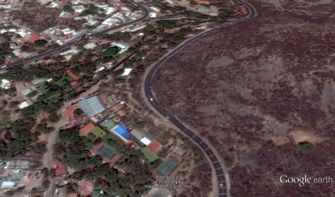
The soil is made up of Feozem (46.1%), Luvisol (28.9%), Cambisol (8.1%), Regosol (4.6%), Acrisol, (4.2%), Leptosol (4.1%) and Vertisol (0.5%), is of the conglomerate subtype. It is reddish, presents sedimentary, igneous, and metamorphic clasts. In the study area it is specifically known that Calcaric Feozem, has some lime less than 50 cm deep with high permeability and medium porosity. A remodeled former hacienda was chosen where the San Juan Nepomuceno Sports Club is located, a family recreation center shown in Figure 1.
Figure 1. Ex Hacienda of San Juan Nepomuceno studied area
Mercury is highly toxic to humans and the environment, its toxicity depends on the bioavailability of its compounds, Mercury in soils is present in two oxidation states: Hg0 y Hg+2 [6, 7], depending on the pH, temperature, and humic content. Methyl mercury is the most toxic compound as it crosses the blood-brain barrier and causes severe neurological problems (irritability, nervousness, tremor, changes in vision and hearing, memory problems, etc.) [8, 9].
Various studies have been carried out on environmental contamination due to mining activity, one is in Slovakia where they found a mercury concentration of 0.28 - 415 mg/kg, these concentrations represent an ecological risk [10, 11].
The official Mexican standard NOM–147–SEMARNAT/SSA1-2004 establishes the concentrations of soils contaminated by arsenic, chromium, and mercury, the total reference concentration (CRt) for mercury for commercial - agricultural - residential use is 23 mg/kg and for industrial use is 310 mg/kg, for soluble mercury contaminants is 0.02 ppm [12].
A study was also carried out on mercury emissions in Peruvian gold stores, mercury oxide concentrations (HgO) were higher than 2,000,000 ng/m3, compared to the case of Guanajuato, the value was higher in the soil surface with 6´1011 ng/m3. A study has been reported on the distribution of Hg in abandoned pond sediments used in small-scale artisanal mining (AGMPs) in San Juan de Choco, Colombia. Total mercury varied in the sediments [13, 14].
Regarding the simulation using CFD for mercury mass transfer in soils and subsoils, there are the following studies. Another study on soil pressure in tillage tools and its distribution on the tool surface are important factors for tool design with regard to tool wear. These factors were investigated using simulations of CFD for high speed tillage. The soil was characterized by its rheological behavior as a Bingham material [15,16].
The present work consists of two objectives:
1. This study aims to determine the concentrations of mercury, a product of the colonial mining activity, in the Hacienda call now Nepomuceno Sports Club.
2. Finding the mathematical model of hydrodynamics and mass transport of mercury in the subsoil to identify the mercury concentration profile using Fluent 16 to validate with the experimental data.
The study of hydrodynamics was carried out with tools of CFD in Fluent 16.0, which will give us the concentration profile of mercury in the soil. A computer with memory was used RAM of 8 GB and a processor AMD A 8.
1.1 Computational model
The following equations are those that are involved in solving the problem posed by the physical phenomenon to be modeled: equation of Reynolds Average Navier-Stokes (RANS), turbulence model $(k-\varepsilon)$ , equations of state, and coupled methods; FLUENT 16TM uses the finite volumes method as a numerical method of solving the governing equations and those mentioned above [17].
The equation of conservation of mass or continuity
$\frac{\partial \rho}{\partial t}+\frac{\partial \rho u_x}{\partial x}+\frac{\partial \rho u_y}{\partial y}+\frac{\partial \rho u_z}{\partial z}=0$ (1)
The Momentum Conservation Equations
Component X
$u_x \frac{\partial u_x}{\partial x}+u_y \frac{\partial u_x}{\partial y}+u_z \frac{\partial u_x}{\partial z}=v\left(\frac{\partial^2 u_x}{\partial x^2}+\frac{\partial^2 u_x}{\partial y^2}+\frac{\partial^2 u_x}{\partial z^2}\right)$ (2)
Component Y
$u_x \frac{\partial u_y}{\partial x}+u_y \frac{\partial u_y}{\partial y}+u_{-} \frac{\partial u_y}{\partial z}=-\frac{\partial p}{\partial y}+v\left(\frac{\partial^2 u_y}{\partial \!x^2}+\frac{\partial^2 u_y}{\partial y^2}+\frac{\partial^2 u_y}{\partial z^2}\right)+\rho g_y$ (3)
Component Z
$u_x \frac{\partial u_z}{\partial x}+u_y \frac{\partial u_z}{\partial y}+u_z \frac{\partial u_z}{\partial z}=v\left(\frac{\partial^2 u_z}{\partial x^2}+\frac{\partial^2 u_z}{\partial y^2}+\frac{\partial^2 u_z}{\partial z^2}\right)$ (4)
The volume of fluid (VOF) multiphase model can model two or more immiscible fluids solving a single set of moment equations and tracking the volume fraction of each of the fluids across the domain.
For this work the Porous Medium Model was also used, this can be used for single phase and multiphase problems, including flow through packed beds, floors and subsoils, filter papers, perforated plates, flow distributors, and tube banks.
It is important to mention that the advection and molecular diffusion of mercury in soil is considered. Mechanical dispersion was also taken into account by the movement of mercury in solution in the porous medium in longitudinal and transverse directions, the longitudinal dispersion due to the width of the channels and the transversal dispersion due to the bifurcation of the roads.
2.1 Experimental sampling
1) The sampling was carried out according to the Mexican standard NMX-AA-132-SCFI- 2006, doing a vertical exploratory sampling, the preparation of the samples consists of the reception, recording, drying, sieving, homogenization, quartering, and storage for their conservation.
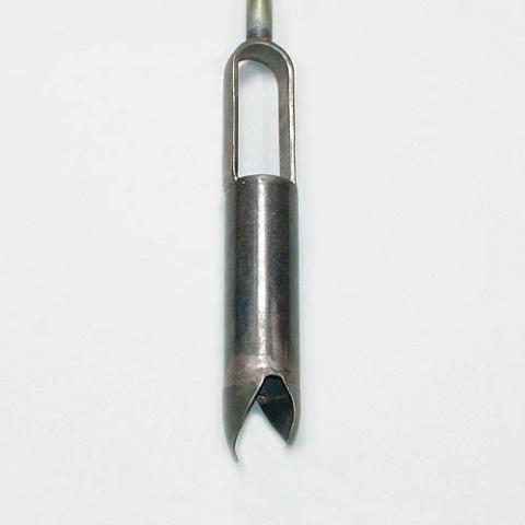
2) The holes in the soil were carried out in the patios of the ex-Hacienda San Juan Nepomuceno, 9 vertical holes were used with a hand auger of type "Riverside" seen in Figure 2, consisting of a 10 cm diameter open tube, with a 2-peaked opening at its base and extendable up to 3 meters, samples were taken at every 10 cm depth, the 9 holes made allowed exploring a depth of between 0.4 to 2.3 meters, analyzing 15 cm of surface soil and discontinuous horizons at depth.
Figure 2. Riverside type hole
3) The acid digestion of the sample was carried out according to the Mexican norm NOM-147-SEMARNAT/SSA1-2004.
4) Was analyzed in the atomic absorption spectrophotometer with cold vapor attachment for mercury analysis, cold vapor generator with mercury gap cathode lamp at a wavelength of 253.7 nm.
2.2 CFD simulation
2.2.1 Preprocessing
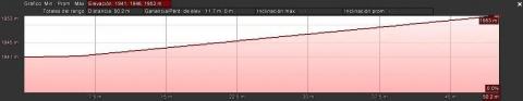
5) First, the terrain and its contour lines were measured, for which the CEM 3.0 was used, which is a program of the INEGI (National Institute of Statistics and Geography).
6) The ArcGis 10.0 program was used to obtain the contour lines to generate the digital elevation model (DEM), see Figure 3.
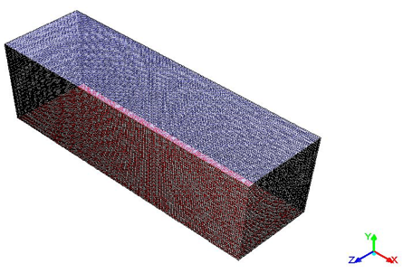
7) Make the geometry CAD in 3 dimensions of the studied area, the dimensions of the land are 5.0 meters long, 2.0 meters wide and 0.15 meters deep.
8) The meshing was carried out in Ansys ICEM software, and the boundary conditions were set.
9) It was malleable with a hexahedral structure with a mesh size of 542750 cells, Figure 4.
Figure 3. Elevation profiles of the area studied in the ex-hacienda Nepomuceno
Figure 4. Mesh generated from the soil to be studied
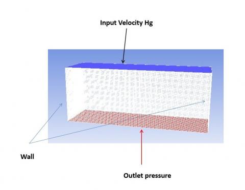
The boundary conditions in the mesh are shown in Figure 5.
Figure 5. The boundary conditions in the mesh
The quality of the geometry meshing was verified with three meshes of hexahedral structure with sizes of 250,300, 542,750 and 980,760 cells. Taking the mesh of 542,750 cells for having little computing power to work.
Table 1. Boundary conditions used in the simulation
|
Boundary conditions |
||||
|
Velocity inlet |
Mass fraction |
Hg volume fraction |
Sand fraction volume |
|
|
Phases |
Mixture |
0.001 |
0 |
0 |
|
Hg |
0.5 |
0 |
0 |
|
|
Sand |
0.5 |
0 |
0 |
|
|
Outlet pressure |
Pressure gauge |
Hg volume fraction |
Sand fraction volume |
|
|
Phases |
Mixture |
0 |
0 |
0 |
|
Hg |
0 |
0 |
0 |
|
|
Sand |
0 |
0 |
0.3 |
|
|
Walls |
||||
|
Phases |
Mixture |
Stationary wall |
||
|
Hg |
0 |
|||
|
Sand |
0 |
|||
2.2.2 Processing
10) The simulation in Fluent 16.0 was carried out in a transitory state, in 3 Dimensions, using the viscous model $k-\varepsilon$ standard with standard wall functions, the VOF multiphase model, with two phases of sand and mercury, with a sparse interface model, and the porous medium model was also used.
The mercury transport phenomenon should be seen as a momentary injection and a convergence criteria of 0.0001 was used to validate the simulation.
11) The boundary conditions used for the simulation in Fluent are shown in Table 1.
12) The mercury flow was 0.0001 m/s, the convergence criteria was 0.001 for all equations, for 4,700 total seconds of simulation.
2.2.3 Post-processing
13) Obtain contours and velocity profiles of mercury transport in the studied terrain, as well as extract graphics and profiles, mercury mass transfer tables (concentrations). It is important to validate the mathematical model, comparing experimental data against simulation data using the tools of Fluent and Results of Ansys.
Initializes with calculated values at the mercury input and from there it is calculated iteratively until meeting the established convergence criteria, which is 0.001 for all equations. The discretization of the equations is second order for the momentum equation and for the turbulence equations.
The solution procedure consisted of activating all the models used from the beginning until all the convergence criteria were met in each of the equations involved, both for transient and steady state regime.
This work presents the results and discussion of the numerical analysis in FLUENT and the experimental results of soil sampling. Hydrodynamic results are presented in soil or mercury diffusion plume in the sampled land of the Ex-Hacienda de San Juan Nepomuceno, velocity magnitude contour is shown, their corresponding vectors, volume fraction contours and mercury concentration profiles at 4700 seconds simulation.
The results made by an atomic absorption spectroscopy analyzer are shown in Table 2, where concentrations with values of 385.4 at 635 ppm of mercury, which is out of the norm.
Table 2. Results of the sampling of mercury in the field
|
Sample |
Weight (g) |
Absorbance |
Blast-hole |
Mercury (ppm) |
|
1 |
0.5 |
0.323 |
S7 |
601.4 |
|
2 |
0.5 |
0.207 |
S9 |
385.4 |
|
3 |
0.5 |
0.238 |
S6 |
443.2 |
|
4 |
0.5 |
0.341 |
S1 |
634.9 |
|
5 |
0.5 |
0.289 |
S3 |
538.1 |
Table 2 shows the values of blast-holes at 0, 5, 10 and 15 cm depth corresponding to 601.4, 385.4, 443.2, 634.9, and 538.1 ppm of Hg experimentally measured in the atomic absorption spectrophotometer, respectively, and where there is a variability between the results and considerable accumulation at 15 cm depth. From the simulation in Fluent, the following results are obtained.
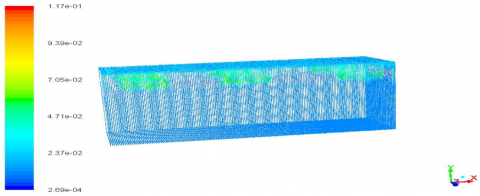
Figure 6 shows the velocity vectors on the ground ranging from a velocity of 0.00237 m/s to a maximum diffusion velocity of 0.0052 m/s within the studied soil, at the beginning the diffusion speed is fast but as it advances in depth it decreases due to the porosity of the sand and the high viscosity of mercury. Therefore, the little movement within the subsoil over the years is evident.
Figure 6. Velocity vectors of the mercury movement in the subsoil
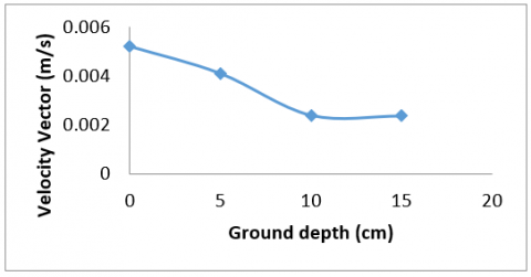
Figure 7 shows the velocity profile towards the interior of the terrain, observing a decrease in speed as shown in the speed vectors, on the surface taking an initial velocity of 0.0052 m/s on the surface at 5 cm a velocity of 0.0041 m/s is noted, at a depth of 10 cm a velocity of 0.0024 m/s, and at 15 cm a value of 0.00237 m/s is observed.
Figure 7. Mercury velocity profile in the depth of the ground
Figure 8 shows the contour of the mercury fraction after 4700 seconds of simulation, where fractions ranging from 0.4 at 0.644 volume fraction of mercury corresponding to concentrations of 400 to 650 ppm of mercury.
Figure 8. Mercury volume fraction contour
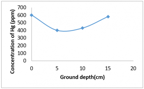
Figure 9 shows the mercury concentration profile in the studied terrain, where the concentration of mercury increases deeper in the subsoil, presented a concentration of 600 ppm of Hg at the soil surface, at 5 cm it decreases to a value of 400 ppm, but at 10 cm it increases to a value of 430 ppm, at a depth of 15 meters the concentration increases to 610 ppm of Hg because there is no longer much diffusion and mercury tends to accumulate in the subsoil.
Figure 9. Hg concentration profile at 4,700 seconds of simulation
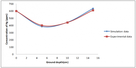
Another important part of the results is how much the mathematical model represents the real phenomenon. Therefore, both results are compared to observe their similarity and it is shown in Figure 10.
Figure 10. Comparison of experimental data (red line) against simulation data (blue line)
Table 3 shows the experimental comparison against the simulation of the mercury concentration in ppm where there is a 4% error rate between the concentrations, varies by trying to compare the porous model with the mean permeability and porosity of the soil and Guanajuato subsoil, since it is never constant, in the porosity model we kept it constant with a value of 0.5 throughout the simulation.
Table 3. Experimental and simulation results of Hg concentration (ppm)
|
Distance |
Hg experimental (ppm) |
Hg simulation (ppm) |
|
0 |
601.4 |
599.5 |
|
5 |
385.4 |
400.24 |
|
10 |
443.2 |
440.3 |
|
15 |
634.9 |
610.35 |
In this work, mercury concentrations were determined via sampling through the Riverside blast - hole and their analysis in the atomic absorption spectrophotometer, shows evidence of anthropogenic mercury contamination in the Ex-Hacienda of San Juan Nepomuceno, where mercury concentrations of 600 ppm exceed up to 20 times the concentrations allowed according to to the norm, which represents a risk to human health in Guanajuato society.
CFD study shows very little mercury diffusion, result of the high porosity and permissibility of the soil of Guanajuato as well as the high density and viscosity of mercury.
According to the Ogata-Banks equation (Banks, 2015), mercury will continue to be transported on the ground, as time passes.
It was also possible to know a value of the transversal dispersion at 3 meters in length and at 15 cm of soil depth, although it had an approximation error of 4% between the experimental and simulation values.
A future work is bioremediation, It is proposed to use several alternatives simultaneously as phytoremediation in combination with some microorganisms associated with plants (rhizoremediation), some plant species have the ability to grow in soils and waters contaminated with heavy metals, and they also have the ability to accumulate a high amount of these substances through physiological adaptations. Some of these plants that can be used to retain mercury are: Limnocharis flava, Thalia geniculate, and Typha latifolia (Anning et al., 2013).
Acknowledgement to Dr. Fabián Salvador Mederos Nieto for his support in the research work, and his research project SIP - IPN 20231028.
|
C |
Constant |
|
C1, C2, C3 |
Constants |
|
gy |
acceleration due to gravity |
|
Gk |
Turbulent kinetic energy generation due to velocity gradients |
|
Gb |
Turbulent kinetic energy generation due to boyance |
|
p |
Pressure (N/m2) |
|
ux |
Fluid velocity in x direction (m/s) |
|
uy |
Fluid velocity in y direction (m/s) |
|
uz |
Fluid velocity in z direction (m/s) |
|
YM |
Contribution of swelling fluctuations in turbulence with dissipation rate |
[1] Ramos, Y.R., Prol-Ledesma, R.M., Siebe-Grabach, C. (2004). Geology and extraction history of the District of Guanajuato. Mexican Journal of Geological Sciences, 21(2): 268-284. https://www.redalyc.org/articulo.oa?id=57221207, accessed on Dec. 23, 2023.
[2] Hylander L.D., Meili M. (2003). 500 years of mercury production: Global annual inventory by región until 2000 and associated emissions. The Science of the Total Environment, 304: 13-27. https://doi.org/10.1016/S0048-9697(02)00553-3
[3] Carrillo Chávez, A., Morton Bermea, O., González-Partida, E., Rivas-Solorzano, H., Oesler, G., Garcı́a-Meza, V., Hernández, E., Morales, P., Cienfuegos, F. (2003). Environmental geochemistry of the mining district of Guanajuato, Mexico. Ore Geology Reviews, 23: 277-297. https://doi.org/10.1016/S0169-1368(03)00039-8
[4] Parsons, M., Percival, J.B. (2005). Mercury sources, measurements, cycles and effects (ed. Parsons, M.B. & Percival, J.B.). Association of Canada; Short Course Series, 34: 1-20. https://www.researchgate.net/publication/264932952_Mercury_Sources_Measurements_Cycles_and_Effects, accessed on Dec. 12, 2022.
[5] Egler, S.G., Rodrigues-Filho, S., Villas-Bôas, R.C., Beinhoff, C. (2006). Evaluation of mercury pollution in cultivated and wild plants from two small communities of the Tapajós gold mining reserve, Pará State, Brazil. Science of the Total Environment, 368: 424-433, 2006. https://doi.org/10.1016/j.scitotenv.2005.09.037
[6] Anning, A.K., Korsah, P.E., Addo-Fordjour, P. (2013). Phytoremediation of wastewater with Limnocharis flava, Thalia geniculata and Typha latifolia in constructed wetlands. International Journal of Phytoremediation, 15(5): 452-464. https://doi.org/10.1080/15226514.2012.716098
[7] Heckel, P.F., Keener, T.C., LeMasters, G.K. (2013). Background soil mercury: An unrecognized source of blood mercury in infants? Open Journal of Soil Science, 3(1): 23-29. https://doi.org/10.4236/ojss.2013.31004
[8] World Health Organization. (1990). Methylmercury: Environmental Health Criteria 101. https://inchem.org/documents/ehc/ehc/ehc101.htm, accessed on Dec 15, 2022.
[9] Musilova, J., Arvay, J., Vollmannova, A., Toth, T., Tomas, J. (2016). Environmental contamination by heavy metals in region with previous mining activity. Bulletin of Environmental Contamination and Toxicology, 97: 569-575. https://doi.org/10.1007/s00128-016-1907-3
[10] Moody, K.H., Hasan, K.M. et al. (2020). Mercury emissions from Peruvian gold shops: Potential ramifications for Minamata compliance in artisanal and small-scale gold mining communities. Enviromental Research. https://doi.org/10.1016/j.envres.2019.109042
[11] Gutiérrez-Mosquera, H., Marrugo-Negrete, J., Díez, S., Morales-Mira, G. Montoya-Jaramillo, L.J., Jonathan, M.P. (2020). Distribution of chemical forms of mercury in sediments from abandoned ponds created during former gold mining operations in Colombia. Chemosfere, 258: 127319. https://doi.org/10.1016/j.chemosphere.2020.127319
[12] NOM–147–SEMARNAT/SSA1-2004. https://www.dof.gob.mx/nota_detalle.php?codigo=4964569&fecha=02/03/2007#gsc.tab=0, accessed on Dec. 15, 2022.
[13] Veiga, M.M., Fadina, O. (2020). A review of the failed attempts to curb mercury use at artisanal gold mines and a proposed solution. The Extractive Industries and Society, 7(3): 1135-1146. https://doi.org/10.1016/j.exis.2020.06.023
[14] Karmakar, S., Kushwaha, R.L. (2006). Dynamic modeling of soil–tool interaction: An overview from a fluid flow perspective. Journal of Terramechanics, 43(4): 411-425. https://doi.org/10.1016/j.jterra.2005.05.001
[15] Guo, Y., Yu, X.B. (2017). Comparison of the implementation of three common types of coupled CFD-DEM model for simulating soil surface erosion. International Journal of Multiphase Flow, 91: 89-100. https://doi.org/10.1016/j.ijmultiphaseflow.2017.01.006
[16] Karmakar, S., Kushwaha, R.L., Lague, C. (2007). Numerical modelling of soil stress and pressure distribution on a flat tillage tool using computational fluid dynamics. Biosystems Engineering, 97(3): 407-414. https://doi.org/10.1016/j.biosystemseng.2007.02.008
[17] ANSYS, Inc. (2017). ANSYS Fluent User's Guide. Canonsburg, PA, USA. http://users.abo.fi/rzevenho/ansys%20fluent%2018%20tutorial%20guide.pdf, accessed on Dec. 25, 2025.