Zhiguang Lan| Wen Zhang* | Guang Yang | Donghui Chen | Junqi Chen
OPEN ACCESS
Determining the critical slip surface of a fractured rock slope remains a major challenge. This study proposes a new method to determine the critical slip surface of fractured rock slope by comprehensively considering fracture characteristics. First, 2D fracture network of main sliding surface is simulated according to the characteristics of fractures on exposed rock surface. Then, potential slip surfaces between different entry and exit points on the main sliding surface are searched by Floyd algorithm. Finally, persistence, i.e. the percentage of total fracture length to the length of potential slip surface, is applied to evaluate the final critical slip surface. According to the above method, the final critical slip surface of a case study was determined, which show that the coordinates of the entry and exit points of the critical slip surface for the fractured rock slope are (62, 86 m) and (14, 30 m), respectively, with the persistence of 85.27 %.
fractured rock slope, critical slip surface, floyd algorithm, persistence
The critical slip surface of a fractured rock slope is mostly controlled by the fractures developed in rock masses [1, 2]. Due to its anisotropy and limitations of measurement, hidden within the rock mass, very little is known about true fractures [3]. Thus, it remains a difficult challenge to determine the critical slip surface of a fractured rock slope.
Presently, researches on critical slip surface of a fractured rock slope are performed using mathematical programming methods and intelligent search algorithms, such as genetic algorithm, colony algorithm, and particle swarm optimization [4-8]. Besides, safety factor with the smallest value is often used as the representative of evaluating critical slip surface. Although many researchers have obtained good results by applying these methods, the following problems remain challenges: (1) these methods usually ignore the presence of fractures or regard fractures as through-going fully persistent planes; (2) it is necessary to obtain the strength parameters (i.e., cohesion and friction angle) of intact rock and fractures for calculating safety factor, which may be not easy to test when the experimental conditions are limited.
In fact, fractures in nature have finite sizes and orientations; therefore, they are often non-persistent. The rational critical slip surface determination should comprehensively consider fractures with finite sizes. Some researchers [9-11] have studied critical slip surfaces by comprehensively considering non-persistent fractures. They tracked slip surfaces at all possible exit points and locate the critical slip surface using intelligent search algorithms. Although these studies attempted to determine critical slip surface, they are inadequate and require further research. Besides, a method of evaluating critical slip surface quickly and accurately when strength parameters are unknown is needed to be recommended.
In the present study, a new method for determining the critical slip surface of fractured rock slope is introduced, which comprehensively considers the location, size, and orientation of each fracture, and regards persistence as index to evaluate the final critical surface.
2.1 Discrete fracture network modeling
A 2D analysis is performed to determine the critical slip surface of fractured rock slope. Before starting the analysis, the fractures on the main sliding surface should be investigated. However, in practice, the fractures on the main sliding surface is usually difficult to investigate. Therefore, it is necessary to simulate and generate the fractures on the main sliding surface on the basis of the fractures on exposed rock surface. The detailed procedures are as follows (Figure 1):
Figure 1. Diagram of discrete fracture network modeling on main sliding surface
2.1.1 3D fracture network modeling
3D fracture network modeling is the most effective method to describe the fractures developed in rock mass, which has become increasingly complete and rigorous for nearly half a century [12, 13]. 3D fracture network can be generated by Monte Carlo simulation, which fits the probability distribution of fracture location, orientation, fracture size, and density on the basis of fractures measured in the field.
The main procedures of 3D fracture network modeling in fractured rock slope are as follows: (1) simulation of fracture location. Generally, the positions of fractures are assumed uniformly random. The simulated fracture locations in 3D space are generated using the Poisson process; (2) simulation of fracture orientation [14-16]. Fractures can be grouped according to statistical homogeneity, and then the average orientation of each group can be determined. Fracture orientation usually obeys Fisher distribution, Bingham distribution, bivariate normal distribution and empirical distribution; (3) simulation of fracture size [17-19]. Up to now, there is no unified conclusion about the shape of the fracture, so it is often assumed that the shape of the fracture is a disk, a polygon, etc. In order to simplify the modeling procedure, the fracture shape is often assumed to be a disk in engineering practice. Assuming that the fracture shape is a disk, the fracture size is characterized by the diameter. Fracture diameter generally obeys normal distribution, lognormal distribution and gamma distribution; (4) determination of fracture density [20-21]. Normal spacing can be obtained by scanline method. Then the volume fracture density can be calculated on the basis of normal spacing using the method proposed by Oda [21]; (5) Monte Carlo simulation [13, 22]. Using Monte Carlo simulation to combine the above parameters, 3D fracture network with similar statistical characteristics to the fractures in the field can be generated.
2.1.2 Generation of fractures on main sliding surface
Assuming that the fracture shape is a disk, the parameters determining the fracture are the center coordinates, diameter, dip direction, and dip angle. The analytical expression of the fracture can be established by these parameters. If the main sliding surface is truncated with the fractures in the 3D fracture network, the fracture trace on the main sliding surface can be determined by the following formula:
$\left\{\begin{array}{c}{A\left(x-x_{c}\right)+B\left(y-y_{c}\right)+C\left(z-z_{c}\right)=0} \\ {\left(x-x_{c}\right)^{2}+\left(y-y_{c}\right)^{2}+\left(z-z_{c}\right)^{2} \leq \frac{D^{2}}{4}} \\ {\cos \theta\left(x-x_{0}\right)+\sin \theta\left(y-y_{0}\right)=0}\end{array}\right.$ (1)
where, D is diameter, (xc, yc, zc) is the center coordinates, θ is the direction of the slope outcrop, and (x0, y0) is the coordinate of any point of the main sliding surface in the 3D fracture network. [A, B, C] is the unit normal vector of the fracture, which can be specifically expressed as [sinβcosα, sinαsinβ, cosβ], where α is the dip direction of the fracture and β is the dip angle of the fracture.
2.2 Floyd algorithm for determining potential slip surface
The potential slip surface mainly extends along pre-existing fractures [1,23]. The more fractures the slip surface passes through, the smaller the shear strength is. When the entry and exit points of a slip surface are fixed, a small total length of the slip surface results in long fractures passed by the slip surface. Thus, when the slip surface is the shortest, the slip surface passes the fractures to the utmost extent, and the shear strength is the smallest [2]. On the basis of this analysis, the potential slip surface of the fractured rock slope extends along the shortest path when the entry and exit points are designated. There are many methods to search the shortest path. Floyd algorithm is easy to understand, and can calculate the shortest distance between any two points. Therefore, Floyd algorithm is used to search the shortest path (i.e., the potential slip surface). Floyd algorithm is introduced as follows [24]:
Two matrices (named D and P, respectively) are needed when calculating the shortest path between points by Floyd algorithm. The element d[i][j] in D represents the distance between point i and point j, the element p[i][j] in P represents the point passing between point i and point j. Assuming that there are N points. Initially, d[i][j] in D is the weight of point i to point j; if i and j are not adjacent, then d[i][j]=∞, and the value of P is j of element p[i][j]. Next, D is updated N times. In the first update, if d[i][j] > d[i][0] + d[0][j] (d[i][0] + d[0][j] denotes the distance between i and j through the first point), then update d[i][j] to d[i][0] + d[0][j], update p[i][j] = p[i][0]. Similarly, if d[i][j] > d[i][k-1] + d[k-1][j], the update d[i][j] is d[i][k-1] + d[k-1][j], p[i][j] = p[i][k-1]. After N updates, the algorithm is completed, and the shortest path of any two points can be obtained by combining D and P.
Figure 2. Example of the search process for the shortest path from a to d using Floyd algorithm
Taking the points shown in Figure. 2 as an example, Floyd algorithm is used to calculate the shortest path between point a and point d. By updating D and P, the shortest path between a and d is a →c→d, and the shortest distance is 3 + 1 = 4.
Floyd algorithm is used in searching the shortest path based on points. However, the fractures on the main sliding surface are straight lines. Therefore, the fractures on the main sliding surface should be initially discretized into several points to execute the searching process. It is noteworthy that many points increase the accuracy of the result of the shortest path but complicate calculations. In addition, in the actual searching process, the entry and exit points of potential slip surface need to be designated beforehand.
2.3 Persistence for evaluating critical slip surface
Fractured rock slope often contains fractures and intact rocks. The shear strength of fractures is one to two orders of magnitude less than that of intact rocks [25-28]. Thus, the characteristics of fractures play an important role in the failure of rock slope. Among these characteristics, persistence, which is known as the areal extent or size of fractures within a rock mass [29], has been recognized as one of the most important parameters that affect the stability in rock slope.
ISRM quantified the persistence as the percentage of the fracture size to a reference size: either the percentage of the sum of the individual fracture areas to the area of a coplanar reference fracture plane; or the percentage of the sum of the trace length to the length of a collinear scanline. This study uses the later concept, that is, defined persistence as the percentage of the sum of the trace length lfi to the length of potential slip surface L.
Researches [30-31] have shown that the greater the persistence is, the lower the shear strength of potential slip surface is, which means that the rock slope is more vulnerable to damage. According to this principle, the potential slip surface with the maximum persistence can be regarded as the critical slip surface.
Taking one fractured rock slope as a case study to determine the critical slip surface by the above methodologies. The fractured rock slope is steep terrain, with elevations ranging from 1359 m to 1481 m. The average orientation of the rock slope surface is 30° ∠ 65°. The dominant rock mass in this slope is diorite composed of white plagioclase and dark amphibole. In addition, due to the long-term influence of geological tectonic movement, the structure of the rock slope is fragmented and fractures are well developed.
Digital close range photogrammetry was used to collect fractures on slope outcrop. The fracture parameters, such as starting point coordinate, terminal point coordinate, dip direction, and dip angle were recorded. Finally, a total of 420 fractures were collected. By using the dynamic clustering method, those fractures were divided into three dominant groups with average orientation of 150° ∠ 80°, 89° ∠ 31° and 339° ∠ 42°. Accordingly, the probability distribution of fracture parameters of each group was determined, as detailed in Table 1.
Table 1. Fracture parameters of each group
|
Fracture group |
Number |
Average orientation |
Trace length |
Density (m-3) |
||||
|
Dip direction (°) |
Dip angle (°) |
Distribution type |
Mean (m) |
Variance (m) |
Distribution type |
|||
|
1 |
176 |
150 |
80 |
Empirical |
4.7 |
12.8 |
Lognormal |
0.0275 |
|
2 |
64 |
89 |
31 |
Empirical |
5.6 |
16.3 |
Lognormal |
0.0110 |
|
3 |
180 |
339 |
42 |
Empirical |
4.4 |
23.6 |
Lognormal |
0.0285 |
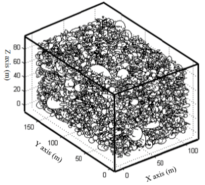
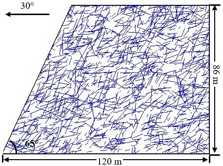
3D fracture network modeling was used to simulate the fractures in the rock slope. Finally, a model with a size of 110 m (X axis) × 170 m (Y axis) × 90 m (Z axis) was generated, and its visualization model is shown in Figure 3. Field investigation shows that the average orientation of the main sliding surface is 30° ∠ 65°. We selected the main sliding surface through the center of the 3D fracture network model, then, fractures on main sliding surface can be generated by Eq. (1). Fractures on the main sliding surface are shown in Figure 4.
Figure 3. Visualizations of the 3D fracture network model
Figure 4. Fractures on the main sliding surface
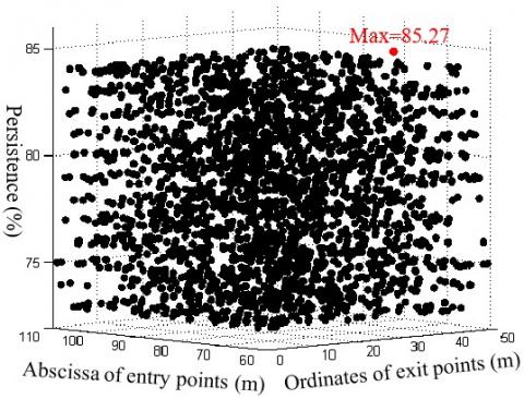
In this study, each fracture trace was uniformly discretized into six points to ensure the search accuracy and reduce the computational complexity. Then, the candidate entry and exit points for locating the potential slip surfaces were set as (x0, 86 m) and (h0/tan65°, h0), respectively. A spacing of 1 m between the adjacent candidate points was set. Finally, 50 different candidate entry points (x0 =61 m, 62 m,…, 110 m) and 50 different candidate exit points (h0 =1 m, 2 m,…, 50 m) were set. A combination of the two series of data results in 2500 sets of entry and exit points, and 2500 potential slip surfaces were found by Floyd algorithm. At the same time, the length of potential slip surface and the total length of fractures were counted, and the corresponding persistence was calculated. The statistical results are shown in Figure 5.
Figure 5. Persistence results of 2500 potential slip surfaces
Figure 6. Final critical slip surface
Statistical results show that the maximum persistence was 85.27 %, and the corresponding potential slip surface is the critical slip surface. Thus, the coordinates of the entry and exit points of the critical slip surface are (62, 86 m) and (14, 30 m), respectively, and the critical slip surface is shown in Figure 6.
According to the method proposed in this study, the critical slip surface of a case study was determined, and the following findings can be drawn.
1) The fractures on the main sliding surface should be generated before conducting the 2D slope analysis. The characteristics (e.g., orientation, size, and density) of the fractures on the main sliding surface are related to those measured on the exposed rock faces. Thus, the fractures on the main sliding surface can be generated through the procedures described in Section 2.1.
2) The potential slip surfaces of the fractured rock slope extend along the shortest path when the entry and exit points are designated. Floyd algorithm can be used to calculate the shortest path between any two points, thereby it can be applied to determine the potential slip surfaces of the fractured rock slope.
3) Different entry and exit points result in different potential slip surfaces. Persistence, i.e. the percentage of total fracture length to the length of potential slip surface, can be used as an index to evaluate the critical slip surface. The coordinates of the entry and exit points of the critical slip surface for the case study are (62, 86 m) and (14, 30 m), respectively, with the persistence of 85.27 %.
This work was supported by the National Nature Science Foundation of China (Grant numbers: 41877220 and 41472243), the National Nature Key Science Program Foundation (Grant number: 41330636), and the National Key Research and Development Plan (Grant number: 2017YFC1501000).
[1] Sharifzadeh, M., Sharifi, M., Delbari, S.M. (2010). Back analysis of an excavated slope failure in highly fractured rock mass: The case study of Kargar slope failure (Iran). Environmental Earth Sciences, 60: 183-192. http://doi.org/10.1007/s12665-009-0178-2
[2] Zhang, W., Zhao, Q.H., Chen, J.P., Huang, R.Q., Yuan, X.Q. (2017). Determining the critical slip surface of a fractured rock slope considering preexisting fractures and statistical methodology. Landslides, 14(3): 1253-1263. http://doi.org/10.1007/s10346-017-0800-4
[3] Shang, J., Hencher, S.R., West, L.J., Handley, K. (2017). Forensic excavation of rock masses: A technique to investigate discontinuity persistence. Rock Mechanics and Rock Engineering, 50(11): 2911-2928. http://doi.org/10.1007/s00603-017-1290-3
[4] Malkawi, A.I.H., Hassan, W.F., Sarma, S.K. (2001). An efficient search method for finding the critical circular slip surface using the Monte Carlo technique. Canadian Geotechnical Journal, 38(5): 1081-1089. http://doi.org/10.1139/t01-026
[5] Chen, C.F., Gong, X.N., Wang, Y.S. (2003). Adaptive colony algorithm and its application to the slope engineering. Journal of Zhejiang University (Engineering Science), 37(5): 566-569. http://doi.org/10.1142/S0252959903000104
[6] Zou, G.D., Jiang, W.Y. (2004). Stability analysis of soil nailing based on coupling algorithm of simulated annealing algorithm and random disposal-method of points. Rock Soil Mech, 25(1): 37-44. http://doi.org/10.2116/analsci.20.717
[7] Sarma, S.K., Tan, D. (2006). Determination of critical slip surface in slope analysis. Geotechnique, 56(8): 539-550. http://doi.org/10.1680/geot.2006.56.8.539
[8] Li, Y.C., Chen, Y.M., Zhan, T.L., Ling, D.S., Cleall, P.J. (2010). An efficient approach for locating the critical slip surface in slope stability analyses using a real-coded genetic algorithm. Canadian Geotechnical Journal, 47(7): 806-820. http://doi.org/10.1139/t09-124
[9] Zhu, D.Y., Qian, Q.H., Zhou, Z.S. (1999). Technique for computing critical slip field of rock slope and its application to design open pit slope. Chin J Rock Mech Eng, 18(5): 567-572. http://doi.org/10.1088/0256-307X/15/12/024
[10] Zhang, W., Chen, J.P., Zhang, W., Lv, Y., Ma, Y.F., Xiong, H. (2013). Determination of critical slip surface of fractured rock slopes based on fracture orientation data. SCIENCE CHINA Technol Sci, 56(5): 1248-1256. http://doi.org/10.1007/s11431-012-5129-6
[11] Xu, Q., Chen, J.Y., Li, J., Yue, H.Y. (2014). A genetic algorithm for locating the multiscale critical slip surface in jointed rock mass slopes. Mathematical Problems in Engineering, (3): 1-10. http://doi.org/10.1155/2014/543081
[12] Priest, S.D. (1993). Discontinuity Analysis for Rock Engineering. Chapman and Hall, London. http://doi.org/10.1016/0926-9851(93)90044-y
[13] Chen, J.P., Xiao, S.F., Wang, Q. (1995). Three dimensional network modeling of stochastic fractures. Northeast norm University Press, Changchun.
[14] Kulatilake, P.H.S.W., Wu, T.H. (1984). Sampling bias on orientation of discontinuities. Rock Mechanics and Rock Engineering, 17: 243-253. http://doi.org/10.1007/bf01032337
[15] Kemeny, J., Post, R. (2003). Estimating three-dimensional rock discontinuity orientation from digital images of fracture traces. Comput Geosci, 29: 65-77. http://doi.org/10.1016/s0098-3004(02)00106-1
[16] Riquelme, A.J., Abellan, A., Tomas, R., Jaboyedoff, M. (2014). A new approach for semiautomatic rock mass joints recognition from 3D point clouds. Comput Geosci, 68: 38-52. http://doi.org/10.1016/j.cageo.2014.03.014
[17] Mauldon, M. (1998). Estimating the mean fracture trace length and density from observations in convex windows. Rock Mechanics and Rock Engineering, 31(4): 201-216. http://doi.org/10.1007/s006030050021
[18] Mauldon, M., Dunne, W.M., Rohrbaugh, M.B. (2001). Circular scanlines and circular windows: new tools for characterizing the geometry of fracture traces. Journal of Structural Geology, 23(2-3): 247-258. http://doi.org/10.1016/s0191-8141(00)00094-8
[19] Zhang, Q., Wang, Q., Chen, J.P., Li, Y.Y., Ruan, Y.K. (2016). Estimation of mean trace length by setting scanlines in rectangular sampling window. International Journal of Rock Mechanics and Mining Sciences, 84: 74-79. http://doi.org/10.1016/j.ijrmms.2016.02.002
[20] Priest, S.D., Hudson, J.A. (1976). Discontinuity spacing in rock. Int J Rock Mech Min Sci Geomech Abstr, 13: 135-148. http://doi.org/10.1016/0148-9062(76)90818-4
[21] Oda, M. (1982). Fabric tensor for discontinuous geological materials. Soil Found, 22: 96-108.
[22] Zhang, W., Chen, J.P., Yuan, X.Q., Xu, P.H., Zhang, C. (2013). Analysis of REV size based on three-dimensional fracture numerical network modelling and stochastic mathematics. Quarterly Journal of Engineering Geology and Hydrogeology, 46: 31-40. http://doi.org/10.1144/qjegh2011-045
[23] Brideau, M., Yan, M., Stead, D. (2009). The role of tectonic damage and brittle rock fracture in the development of large rock slope failures. Geomorphology, 103: 30-49. http://doi.org/10.1016/j.geomorph.2008.04.010
[24] Qiu, X.P., Wang, L.J. (2019). Research on Shortest Path Optimization Based on Floyd Algorithm. Journal of Taiyuan Normal University (Natural Science Edition), 18(2): 53-56.
[25] Park, H.J. (2005). A new approach for persistence in probabilistic rock slope stability analysis. Geosciences Journal, 9: 287-293. http://doi.org/10.1007/bf02910589
[26] Kemeny, J. (2005). Time-dependent drift degradation due to the progressive failure of rock bridges along discontinuities. International Journal of Rock Mechanics and Mining Sciences, 42: 35-46. http://doi.org/10.1016/j.ijrmms.2004.07.001
[27] Hencher, S., Richards, L.R. (2014). Assessing the shear strength of rock discontinuities at laboratory and field scales. Rock Mechanics and Rock Engineering, 48(3): 883-905. http://doi.org/10.1007/s00603-014-0633-6
[28] Tuckey, Z., Stead, D. (2016). Improvements to field and remote sensing methods for mapping discontinuity persistence and intact rock bridges in rock slopes. Engineering Geology, 208: 136-153. http://doi.org/10.1016/j.enggeo.2016.05.001
[29] ISRM (International Society for Rock Mechanics). (1978). Suggested methods for the quantitative description of discontinuities in rock masses. International Journal of Rock Mechanics and Mining Sciences & Geomechanics Abstract, 15: 319-368. http://doi.org/10.1016/0148-9062(79)91476-1
[30] Chen, J.P., Lu, B., Gu, X.M., Fan, J.H. (2005). Determining 3D persistence of rock mass discontinuity by projection. Chinese Journal of Rock Mechanics and Engineering, 24(15): 2617-2621. http://doi.org/1000-6915(2005)-2617-05
[31] Lu, B., Chen, J.P., Shi, B.F. (2004). Application of genetic algorithm to the determination of 3D persistence of jointed rock mass. Chinese Journal of Rock Mechanics and Engineering, 23(20): 3470-3474. http://doi.org/1000-6915(2004)20-3470-05