Xuxia Deng | Huimin Chen* | Yunbao Xu
OPEN ACCESS
The relationship of foreign trade and forest degradation is an important research topic in trade and environment. Based on dynamic optimal control method, the interrelation of forest resources’ stock dynamic and foreign trade, market power and foreign debt or asset, is exploited. At the same time, the condition and change law of forest degradation is analyzed. Pontryagin Maximum Principle demonstrate a character which if shadow social price of forest resource has a higher price than, demand of forest resource exceed the supply, forest resource decreases, hence lead to forest degradation, even extinction. Some conditions are satisfied, the stock of forest resource and trade terms change in the same direction, and the stock of forest resources and market power varied in same direction. Existing foreign debts, and the international capital market, stock of forest resources will not be dried up.
Pontryagjin maximum principal, foreign debt, market power
Forest resource is a renewable resource, with the economic value and the important ecological value of purifying the air, carbon sequestration, conserving soil and water, tourism etc. Foreign trade has direct or indirect impacts on the domestic and global forest resource stock by technology effect, scale effect, etc. When the exploitation goes faster than the renewal of forest resource, forest resource would come to degradation.
The forest resource assessment 2010 report released from The United Nations Food and Agriculture Organization shows from 1990 to 1999, about 16 million hectares of forest area in the world were destroyed each year, and in 2000-2009, about 13 million hectares were destroyed each year [1]. In 2013 the report from the World Resources Institute states 30% of the world's forests have been cleared, 20% of the forests are in a state of degradation, and 35% of the forests have been in fragmentation [2]. The overall degradation of global forest resource has slowed down, but global forest resource trade keeps growing, for instance, the global import and export of forest goods reached about $454.1 billion in 2010, about $511.1 billion in 2014, with an average annual increase of about $14 billion. From a global perspective, there is a positive correlation between international trade and degradation of forest resource, but how international trade influences forest degradation lacks mathematical analysis. Thus, the research will be developed in this paper based on it.
The researches in the important literature are mainly developed from two aspects. The first is that foreign trade's impacts on logging. Under certain conditions international trade can result in increasing or decreasing of logging, for instance, Shimamoto et al. [3] demonstration on the relationship between forest good trade and logging in Philippines, Thailand, Indonesia proved that the increase of free trade can result in the growth of logging. Jinji [4] in his study found free trade leads to the increase of resource stock in the forest resource-abundant countries, and the decrease of resource stock in the forest resource-poor countries; Tsurumi and Managi [5] in his study found that the openness to the world has a positive correlation to logging sponsored by the organization for economic cooperation and development, but a negative correlation to logging from the organization for non-economic cooperation and development. The second is that the impacts of the factors influencing international trade on logging. Shimamoto [6] thinks imposing import and export duties and domestic price support policy can maintain the sustainable development of forest resource. Capistrano and Kiker [7] and Kahn and McDonald [8] concluded from their researches that there is a positive correlation between foreign debt and logging. The results from Arcand et al. [9] and Richards et al. [10] show that the depreciation of exchange rate can lead to the growth of logging.
Most literature focused on renewable resources as a whole object, thereby ignored the characteristics of the individual; furthermore, the previous researches point out that it is only in the especial case that excessive exploitation may occur, but in the present situation resource functions are weakening everywhere. Therefore, this article focuses on forest resource on the basis of the previous researches.
The main literature closely related to this study are [11-13].
Referring to resource good as consumer good and intermediate good, Kemp and Suzuki [11] studied the optimal conditions of the renewable resources on renewal rate, trade, production and social effects in small countries, and the model results of the optimal conditions show that renewable resources can be sustainably developed, but relaxed conditions may also lead to resource exhaustion. Kemp and Suzuki [11] introduce the linear form of renewable resources to recover production function, and greatly simplify the original and extended model of Faustmann without loss of generality, thereby provides a processing tool for this study. Kemp and Suzuki [11] introduction of intermediate good brings about the complexity of the problem analysis, however, not considering the intermediate good has not a material impact on the result of problem analysis. Thus, based on Kemp and Suzuki [11] analysis, the forest resource good is directly referred to as the final consumer good without intermediate good in this study.
McRAE [12] analyzed renewable resources dynamic by introducing a supply curve function linking to import and export (1978), and adopting the greatest social effects as constraint to conclude that the renewable resources stock level in the optimal steady state is higher than a short-sighted steady-state level and the resources development is sustainable. One of the striking features of McRAE theoretical model is that the effective resource stock is referred to as the effectiveness parameters of next resource stock, which is convenient, general, and provides the reference for this study.
Barbier and Rauscher [13] studied the dynamic problems of the optimal production, consumption, trade of the tropical rain forest resource with the constraint by introducing positive externality of tropical rain forest and setting the maximization goal of social effects on the premise of only producing forest good. The research results show the tropical rain forest resource is sustainable in the long term. Barbier and Rauscher only took a single professional production mode into account so that it is hard to give clear explanation for economic phenomena, therefore, the diversified production mode is introduced.
Kemp and Suzuki [11] and McRAE [12] did not take externalities of renewable resources stock into consideration, and Barbier and Rauscher [13] did not consider the artificial restoration effects on forest resource, so, to a certain extent, the three core literature simplified the actual situation of forest resource development and restoration, and their conclusions have obvious differences. Aside from forest resource supplying directly forest good, the positive externality of its stock has attracted more and more attention. High stock of forest resource can promote the tourism service value, purify groundwater and air ,and improve the life quality of citizens; other positive externalities of forest resource high stock, such as preventing water loss and soil erosion and maintaining biodiversity, are often ignored.On the basis of the research tools and innovations provided in the three core literature by Kemp and Suzuki [11] and McRAE [12] and Barbier and Rauscher [13], combined with the theoretical basis in literature review, and using the dynamic optimization theory, this paper studies the dynamic impacts of foreign trade on forest resource by setting the maximization goal of social consumption in considering artificial restoration of forest resources and the positive externality of forest resource stock so as to draw a more general conclusion.
3.1 Basic assumptions
Hypothesis 1 There are three sectors -- forest resource exploitation, industry and forest resource recovery. Forest resource exploitation sector, abbreviated as resource sector, depends on labor and forest resource stock; Forest resource recovery sector (recovery sector) and industrial sector only need labor.
Hypothesis 2 produce two goods of resource good and manufactures good, and participate in international trade. Both resource and manufactures circulate in consumption field as a final product.
Hypothesis 3 Two countries: the host country and the foreign country. The host country, which exports resource good, and imports manufactures, is the recipient of the international market price.
Hypothesis 4 A labor input factor, with the constant total, homogeneity and full employment. Labor can be understood as effective labor, that is, the fusion of labor and capital.
Hypothesis 5 Forest resource of private property rights have homogeneity, and the development of the forest resource can only obtain competitive profit.
Hypothesis 6 Full competition and complete information.
Hypothesis 7 No transaction costs and no international transport cost.
Hypothesis 8 Trade balance: the import value equals to the export value.
3.2 Production and trade
3.2.1 Resource sector production
Resource sector supplies resource good by the labor and forest resource stock for domestic consumption and export. Resource sector can be understood as agriculture department including the non-forest and forest resource good, which makes feasibility stronger because of the conflict between the utility of agricultural land and forest land. Resource sector production function takes the form of Plourde [14], McRAE [12] form, similar to the C - D (Cobb - Douglas production function) production function, specified as
$Q_{f}=G\left(N_{f}, S\right)$ (1)
$G(\cdot)$ is a function of the resource good production; $Q_{f}$ is the domestic resource good; $N_{f}$ is the amount of labor used in resource sector; $\mathrm{X}$ is the forest resource stock used in the resource good production. The function of resource good production is a quasi-concave function, satisfying the Paddy Conditions (Inada Conditions), with production technology satisfying the strictly increasing conditions, as given by $G_{1}>$ $0, G_{11}<0$ and $G_{2}>0, G_{22}<0(1,2$, respectively stand for $N_{f}$ and $\left.\mathrm{S}\right), G_{12}>0$ (it is defined as a complementary relationship between labor and resources stock, see Venek [15]).
3.2.2 Industrial sector production
Industrial sector produces industrial good for domestic consumption only by labor, otherwise, by import. To simplify the analysis, take the labor as a capitalized composite labor and the general production function is formulated as:
$Q_{i}=F\left(N_{i}\right)$ (2)
$F(\cdot)$ is the production function of industrial sector; $Q_{i}$ is the industrial good yield for domestic consumption; $N_{i}$ is the amount of labor used in industrial sector. The production function of industrial sector satisfies the quasi concave and is continuously differentiable, namely, subject to the conditions given by $F^{\prime}>0, F^{\prime \prime}<0$, and $F(0)=0$.
3.2.3 Recovery production sector
Kemp and Suzuki [11] take the linear form of the production function, such as $Q_{r}=R\left(N_{r}\right)=R\left(N-N_{f}-N_{i}\right) \cdot R(\cdot)$ is the production function of recovery sector, $Q_{r}$ is the yield in recovery sector, $\mathrm{N}$ is the total amount of population; Faustmann [16] analyzed the forest resource dynamic by means of tree-age structure. Usually, while exploiting, the resource sector recovers forest regardless of the forest treeage's dynamic structure, which distinguishes from Faustmann [16] and the extension of literature based on it (such as Clark and Shrestha [17]). It is assumed that the resources recovery yield is a fixed proportion $\theta$ (stands for the output coefficient of resource recovery), specified as
$Q_{r}=\theta \cdot Q_{f}=\theta \cdot G\left(N_{f}, S\right)$ (3)
3.2.4 Foreign trade relations
With the combination of hypothesis 3 , hypothesis 6 , and hypothesis 8 , the resource good export is associated with the manufactures import in quantity, as given by $P_{f w} E_{f}=P_{i w} I_{i}$. $P_{f w}$ is the international price of resource good, $E_{f}$ is the volume of resource good export, $P_{i w}$ is the import price of manufactures, and $I_{i}$ is the volume of resource good import.
Define the terms of trade as $P_{w}=P_{f w} / P_{i w}$, and the relation between import and export trade volume is presented by the following:
$I_{i}=\left(P_{f w} / P_{i w}\right) \cdot E_{f}=P_{w} \cdot E_{f}$ (4)
The relationship between import and export in resource good and manufactures can also be concluded from the implied relationship in supply curve. If interested, see page 32 of McRAE [12] literature.
3.2.5 Equilibrium equation
From 3.2.1 to 3.2.4, the equilibrium equation and dynamic equation can be gotten as follows:
$N=N_{f}+N_{i}$ (5)
$\dot{S}=X(S)+Q_{r}-G\left(N_{f}, S\right)$ (6)
$C_{f}=Q_{f}-E_{f}=G\left(N_{f}, S\right)-E_{f}$ (7)
$C_{i}=Q_{i}+I_{i}=F\left(N_{i}\right)+P_{w} \cdot E_{f}$ (8)
$X(S)$ represents the natural growth function of forest resource, and follows the change law of the Logistic function $[18-20]$, as given by $X(0)=N(\bar{S})=0,0<S<\bar{S}, X(S)>$ $0, X^{\prime \prime}(S)<0 . \dot{S}(t)=d S / d t$ denotes the forest resource growth, and time identifier will be omitted in the subsequent analysis. If $\dot{S}>0$, the increase of forest resource stock can be understood as a kind of positive capital investment; If $\dot{S}<0$, the decrease of forest resource stock can be understood as a kind of negative capital investment. $C_{f}, C_{i}$ are the domestic consumption quantity of resource good and manufactures, respectively. Eq. (5) represents the employment distribution in three sectors; Eq. (6) represents the dynamic change of forest resource stock in consideration of resource good production and resources recovery; Eq. (7) stands for the equilibrium relationship of domestic forest resource consumption in consideration of resource good export; Eq. (8) stands for the equilibrium relationship of domestic manufactures consumption in consideration of manufactures import.
3.3 Social welfare function
Introducing the production, import and export, consumption to the objective of social welfare function maximization is more conducive to analysis on dynamic changes of forest resource, and the specified social welfare function is
$U=U\left(C_{f}, C_{i}, S\right)=U\left(C_{f}\right)+U\left(C_{i}\right)+U(S)$ (9)
The instantaneous social welfare function is subject to the separable additive property and $U_{i}=\partial U / \partial i, U_{i i}=\partial^{2} U / \partial i^{2}$, $U_{i j}=\partial^{2} U / \partial i \partial j, 1$ stands for $C_{f}, 2$ stands for $C_{i}, 3$ stands for $S, U_{i}>0, U_{i i}<0, U_{i j}=0 .$
3.4 Optimal objective and constraints
For export of resource good, import of manufacturers, and policy for social welfare maximizing in the host country, it can be expressed as the formula:
$W\left(C_{f}, C_{i}, X\right)=\int_{0}^{\infty} U\left(C_{f}, C_{i}, X\right) \cdot e^{-\delta t} d t$ (10)
Transpose and sort the formulas from (5) to (8), and get the constraint conditions:
$W\left(C_{f}, C_{i}, X\right)=\int_{0}^{\infty} U\left(C_{f}, C_{i}, X\right) \cdot e^{-\delta t} d t$ (11)
$F\left(N_{i}\right)+P_{w} \cdot E_{f}-C_{i}=0$ (12)
$N-N_{f}-N_{i}=0$ (13)
$\dot{S}=X(S)-(1-\theta) G\left(N_{f}, S\right)$ (14)
$S(0)=S_{0}, \lim _{t \rightarrow \infty} S(t) \geq 0, S^{\max }>S^{\min } 0, X\left(S^{\max }\right)=$$X\left(S^{\min }\right), X^{\prime \prime}(S)<0$ (15)
Symbol description: omit time identifier t; the corresponding functions are denoted by letters; the numbers below letters denote partial derivative; the dots over letters denote time differential; the superscript apostrophes of letters denote derivation N-Nf-Ni=0.
4.1 Dynamic equation of forest resource
According to the Pontryagin Maximum Principle,(PMP: Pontryagin Maximum Principle), it is concluded that if the optimal control variables $C_{f}^{*}, C_{i}^{*}, S^{*}, N_{f}^{*}, N_{i}^{*}, N_{r}^{*}$ in (10) subject to the conditions from (11) to (15) are satisfied, the instantaneous Maximum effects conditions including an adjoint variable and three Lagrange multipliers can also be satisfied, then the current value of Hamilton function (current valued Hamiltonian function) and Lagrangian function (Lagrangian function) are as follows:
The current value of Hamilton function is $H=$ $U\left(C_{f}, C_{i}, S\right)+\lambda \cdot\left(X(S)-(1-\theta) G\left(N_{f}, S\right)\right) .$
Lagrangian function is $L=H+b_{1}\left(G\left(N_{f}, S\right)-E_{f}-C_{f}\right)+$ $b_{2}\left(F\left(N_{i}\right)+P_{w} \cdot E_{f}-C_{i}\right)+b_{3}\left(N-N_{f}-N_{i}\right) . \lambda$ is an adjoint variable, and represents the shadow price current value of forest resource as an investment; $\lambda\left(X(S)+\theta \cdot N_{r}-G\left(N_{f}, s\right)\right)$ is the current value of future utility resulting from the increase or decrease of forest resource as an investment; $H$ is the current value of the total utility of consumption, consisting of the instantaneous direct utility and positive (negative) instantaneous indirect utility after the future utility liquidation resulting from the increase or degradation of forest resource as an investment; $L$ is the Lagrangian function subject to constraints (11) to (14).
The necessary conditions to be satisfied for the optimal control solution are as follows:
$U_{1}=b_{1}$ (16)
$U_{2}=b_{2}$ (17)
$\mathrm{U}_{3}=-\lambda X^{\prime}-\left(b_{1}-\lambda(1-\theta)\right) G_{2}$ (18)
$b_{1} / b_{2}=P_{w}$ (19)
$\left(b_{1}-\lambda(1-\theta)\right) G_{1}=b_{2} F^{\prime}=b_{3}$ (20)
$b_{1}, b_{2}$ are respectively defined as the the marginal value or shadow price of forest resource good and manufactures (or the user cost); $b_{3}$ is the implied labor wage.
Eqns. (16) and (17) denote that the marginal utility from the consumption of resource good, manufactures equals to their own shadow price (or the user cost); Eq. (18) denotes that the marginal social utility of forest resource stock equals to the sum of shadow price from giving up resource exploitation and the user cost resulting from the decrease of resource good production; Eq. (19) denotes the implied resource good price rate equals to the international resource good conversion rate (terms of trade, that is, the resource good conversion ratio from trade between the host country and the foreign country); Eq. (20) denotes that the marginal product value of resource good and manufatures equals to the implicit labor wage, in which $b_{1}-\lambda(1-\theta)$ is the resource good production input price after the deduction of the resource usage cost. The following equation can be obtained by transformation.
$U_{1} / U_{2}=b_{1} / b_{2}=P_{w}=\frac{F^{\prime}}{G_{1}}\left(\frac{b_{1}}{b_{1}-\lambda(1-\theta)}\right)$ (21)
The Pontryagin Maximum Principle determines the dynamic characteristics of the adjoint variable, namely,
$\dot{\lambda}=\lambda \cdot\left(\delta-X^{\prime}+G_{2}(1-\theta)\right)-b_{1} G_{2}-U_{3}$ (22)
Proposition 1 The change rate of social shadow price of forest resource at the time direction $(\lambda)$ equals to the opportunity cost of holding unit forest resource $\left(\lambda\left(\delta-X^{\prime}+G_{2}(1-\theta)\right)\right.$ minus the sum of marginal product value of resources production $\left(b_{1} G_{2}\right)$ and social value of the resource stock $U_{3}$.
4.2 Two important implicit functions
Rewrite Eqns. (16) and (17) by (7) and (8), then the following equations are obtained:
$b_{1}=U_{1}\left(C_{f}\right)=U_{1}\left(G\left(N_{f}, S\right)-E_{f}\right)$$=U_{1}\left(G(f(S, \lambda), S)-E_{f}\right)$ (23)
$b_{2}=U_{2}\left(C_{i}\right)=U_{2}\left(F\left(N_{i}\right)+P_{w} E_{f}\right)$$=U_{2}\left(F(N-f(S, \lambda))+P_{w} E_{f}\right)$ (24)
Two differential Eqns. (14), (22) and five variables $\left(N_{f}, N_{i}, E_{f}, S, \lambda\right)$ constitute the dynamic system. It is feasible to reduce five variables to two variables by using full employment conditions (5) and two implicit relation equations.
Substituting (23) and (24) into (20) yields
$\begin{aligned}\left\{U_{1}\left[G\left(N_{f}, S\right)-E_{f}\right]\right.&-\lambda(1-\theta)\} G\left(N_{f}, S\right) \\ &-\left\{U_{2}\left[F\left(N-N_{f}\right)-P_{w} E_{f}\right] F^{\prime}\left(N-N_{f}\right)\right\} \end{aligned}$ (25)
Eq. (25) implies the relationship between $N_{f}, E_{f}, S, \lambda$. $D\left(N_{f}, E_{f}, S, \lambda\right)$ is defined as the first implicit function relation equation.
Substituting (19) into (23) and (24) yields
$U_{1}\left[G\left(N_{f}, S\right)-E_{f}\right]-P_{w} U_{2}\left[F\left(N-N_{f}\right)-P_{w} E_{f}\right]=0$ (26)
The second implicit function relation equation $B\left(N_{f}, E_{f}, S\right)$ is defined by Eq. (26).
The first and second implicit function incorporate the relationship between employment, export and forest resource, social shadow price.
4.3 Labor allocation, export in resource sector and resource dynamics
Eqns. (4) and (5) show that the labor allocation and export in resource sector determine the labor allocation and import in the industrial sector. Jacobian coefficient can be obtained from finding the derivatives of Eqns. (25) and (26), and here 1, 2, 3, 4 are used as subscripts for convenience, then it results the following equations:
$D_{1}=U_{11} G_{1} G_{1}+\left[U_{1}-\lambda(1-\theta)\right] G_{11}+U_{22} F^{\prime} F^{\prime}$$+U_{2} F^{\prime \prime}$ (A1)
$D_{2}=-U_{11} G_{1}-U_{22} P_{w} F^{\prime}$ (A2)
$D_{3}=U_{11} G_{2} G_{1}+\left[U_{1}-\lambda(1-\theta)\right] G_{12}$ (A3)
$D_{4}=-(1-\theta) G_{1}$ (A4)
$B_{1}=U_{11} G_{1}+U_{22} F^{\prime} P_{w}$ (A5)
$B_{2}=-U_{11}-P_{w} U_{22} P_{w}$ (A6)
$B_{3}=U_{11} G_{2}$ (A7)
$B_{4}=0$ (A8)
It can be known from the model setting as follows: $U_{1}>$$0, U_{2}>0, G_{1}>0, G_{2}>0, P_{w}>0, F^{\prime}>0, \quad$ and $U_{11}<$$0, U_{22}<0, G_{11}<0, G_{22}<0, F^{\prime \prime}>0, \quad U_{1}-\lambda(1-\theta)>$$0, G_{12}>0$,therefore, $D_{1}<0, D_{2}>0, D_{3} \gtreqless 0, D_{4}<0 ; B_{1}<$$0, B_{2}>0, B_{3}<0, B_{4}=0$.
$N_{f}, E_{f}$ Function expression can be gotten from
$J=\left|\begin{array}{cc}\frac{\partial D}{\partial N_{f}} & \frac{\partial D}{\partial E_{f}} \\ \frac{\partial B}{\partial N_{f}} & \frac{\partial B}{\partial E_{f}}\end{array}\right|=\left|\begin{array}{ll}D_{1} & D_{2} \\ B_{1} & B_{2}\end{array}\right|=D_{1} B_{2}-D_{2} B_{1}<0$
specified as followed.
$N_{f}=f(S, \lambda)$ (27)
$E_{f}=h(S, \lambda)$ (28)
Take the derivative of (27), (28), and get
$f_{1}=\frac{1}{-J}\left[\begin{array}{ll}D_{3} & D_{2} \\ B_{3} & B_{2}\end{array}\right]=\frac{1}{-J}\left(D_{3} B_{2}-D_{2} B_{3}\right)$ (A9)
$f_{2}=\frac{1}{-J}\left[\begin{array}{ll}D_{4} & D_{2} \\ B_{4} & B_{2}\end{array}\right]=\frac{1}{-J}\left(D_{4} B_{2}-D_{2} B_{4}\right)$ (A10)
$h_{1}=\frac{1}{-J}\left[\begin{array}{ll}D_{1} & D_{3} \\ B_{1} & B_{3}\end{array}\right]=\frac{1}{-J}\left(D_{1} B_{3}-D_{3} B_{1}\right)$ (A11)
$h_{2}=\frac{1}{-J}\left[\begin{array}{ll}D_{1} & D_{4} \\ B_{1} & B_{4}\end{array}\right]=\frac{1}{-J}\left(D_{1} B_{4}-D_{4} B_{1}\right)$ (A12)
It can be known from the value of D and B in formulas(A1-A8) as $f_{2<0}, h_{2}<0, f_{1} \gtreqless 0, h_{1} \gtreqless 0$.
Substitute (27), (28) into (20), and find the derivative of social shadow price of forest resource to obtain:
$\begin{aligned} \frac{\partial C_{f}}{\partial \lambda}=\frac{\partial[F(f(S, \lambda), s)-h(S, \lambda)]}{\partial \lambda} &=G_{1} f_{2}-h_{2} \\ &=\frac{1}{-J}\left[\left(G_{1} P_{w}-F^{\prime}\right)(1-\theta) G_{1} P_{w} U_{22}\right]<0 \end{aligned}$ (A13)
From (20), obtain
$F^{\prime}=\left(\frac{U_{1}}{U_{2}}\right) G_{1}-\frac{\lambda(1-\theta)}{U_{2}} G_{1}$ (A14)
Both sides of (19) are multiplied by G1 to derive:
$\left(\frac{U_{1}}{U_{2}}\right) G_{1}=P_{w} G_{1}$ (A15)
from (A14) and (A15), concluded as $P_{w} G_{1}>F^{\prime}$, therefore,
$P_{w} G_{1}-F^{\prime}>0$ (A16)
The conclusion of (A13) can be drawn from (A16), namely, (A1-A8).
The relationship between resource dynamic and labor allocation, export in resource sector is given in (A10), (A12), (A13), (A17).
$\frac{\partial C_{i}}{\partial \lambda}=\frac{\partial\left[F(N-f(S, \lambda))+P_{w} h(S, \lambda)\right]}{\partial \lambda}=F^{\prime} f_{2}+P_{w} h_{2}$$=\frac{1}{-J}(1-\theta)\left[\left(F_{2}^{\prime}+P_{w} h_{2}\right) U_{11}\right.$$\left.+2 F_{2}^{\prime} P_{w} U_{22} P_{w}\right]<0$ (A17)
Proposition 2 When the optimal control value $\left(C_{f}^{*}, C_{i}^{*}, N_{f}^{*}, N_{i}^{*}, E_{f}^{*}\right)$ is in the optimal control path, $f_{2}, h_{2}$ must be negative, the social shadow price of forest resource stock increases, the labor force allocated to the resource sector decreases, and the resource good output declines; the labor force allocated to the industrial sector increases, the manufactures production grows up, the resource good export decreases, and the manufactures import declines; thereby, the total consumption of resource good and manufactures absolutely declines; forest resource is well protected. On the contrary, the decrease of social shadow price of forest resource can result in the forest degradation.
Proposition 3 When the optimal control value $\left(C_{f}^{*}, C_{i}^{*}, N_{f}^{*}, N_{i}^{*}, E_{f}^{*}\right)$ is in the optimal control path, due to $D_{3} \gtreqless 0$, then $f_{1} \gtreqless 0, h_{1} \gtreqless 0$, namely, the output, import, export and consumption of resource good and manufactures present different rules.
This means there are four kinds of situation: the first is $f_{1}>$ $0, h_{1}>0$, that is, when the forest resource stock increases, the labor force allocated to the resource sector increases, resource good output grows up, and the export increases; the manufactures import increases, and the manufactures output decreases; Due to the conversion effect of domestic output, import and export, it is uncertain whether the absolute consumption of resource good and manufactures increase, decrease or keeps fixed.
The second is $f_{1}<0, h_{1}<0$, that is, when the forest resource stock increases, labor force allocated to the resource sector decreases, resource good output is uncertain (because the increase and decrease of $\mathrm{S}$ have complementary relationship), and the export declines; the labor force allocated to the industrial sector increases, the output grows up, and import declines; it is uncertain whether the absolute consumption of resource good and manufactures is increasing, decreasing or constant.
The third is $f_{1}>0, h_{1}<0$, that is, when the forest resource stock increases, the labor force allocated to the resource sector increases, output grows up, and exports declines; the labor force allocated to the industrial sector decreases, and the output falls; the resource good consumption increases, and the manufactures consumption falls.
The fourth is $f_{1}<0, h_{1}>0$, that is, when the forest resource stock increases, the labor force allocated to the resource sector decreases, the resource good output is uncertain(because the increase and decrease of $\mathrm{S}$ have complementary relationship), and the export increases; the labor force allocated to the industrial sector decreases, the output falls, and the import increases; the absolute consumption of resource good increases, and the absolute consumption of manufactures good is uncertain.
4.4 Dynamic rule of resource in steady state
The differential equation of (14) and (22) satisfying the initial conditions of equation (15) describes the optimal change at time direction. To have a dynamic analysis, substituting (27) and (28) finds:
$\dot{S}=X(S)-(1-\theta) G[f(S, \lambda), S)$ (29)
$\begin{aligned} \dot{\lambda}=\lambda\left\{\delta-X^{\prime}\right.&\left.(S)+(1-\theta) G_{2}[f(S, \lambda), S)\right\} \\ &-U_{1}\{G[f(S, \lambda), S]\\ &-h(S, \lambda)\} G_{2}[f(S, \lambda), S)-U_{3}(S) \end{aligned}$ (30)
Eqns. (29) and (30) implies the relationship between supply and demand of the forest resource. A detailed analysis on it will be in the following.
4.4.1 The steady-state forest resource demand curve
Eq. (30) implies the forest resource demand curve. From the form, it seems hard to analyze the solution of the specific function, but the trend of the change can be judged by calculating the slope $\partial \lambda / \partial S$. Define $Z(S, \lambda)=0$ as the implicit function of $\dot{\lambda}=0$ (the demand curve of resource), then, $\frac{\partial \lambda}{\partial s}=$ $-Z_{S} / Z_{\lambda}$. Define $Z(S, \lambda)$ as rewritten by
$\begin{aligned} Z(S, \lambda)=\lambda\{\delta&\left.-X^{\prime}(S)+(1-\theta) G_{2}[f(S, \lambda), S]\right\} \\ &-U_{1}\{G[f(S, \lambda), S]\\ &-h(S, \lambda)\} G_{2}[f(S, \lambda), S)-U_{3}(S) \end{aligned}$
Find the derivation of $\lambda, S$ to obtain the expression equation of $Z_{\lambda}, Z_{S}$ respectively:
(1) $\quad Z_{\lambda}=\left(\delta-X^{\prime}\right)+\left\{\left[\lambda(1-\theta) G_{21}-U_{11} G_{1} G_{2}\right] f_{2}+\right.$ $\left.U_{11} G_{2} H_{2}\right\}-U_{1} G_{21} f_{2}+(1-\theta) G_{2}$, analyze $Z_{\lambda}$ as follows:
1) $\delta-X^{\prime}>0$.If $\dot{\lambda}=0$, rewrite (22) as $\delta-X^{\prime}=$ $\frac{\left(b_{1}-\lambda(1-\theta)\right) G_{2}}{\lambda}+\frac{U_{3}}{\lambda}$, which is the output price of forest resource good and must be greater than zero, so $b_{1}-\lambda(1-\theta)$ must be greater than zero, then $\delta-X^{\prime}>0$.
2) $-U_{1} G_{21} f_{2}>0$.Because of $U_{1}>0, G_{21}>0, f_{2}<0$, so $-U_{1} G_{21} f_{2}>0$
3) $\left\{\left[\lambda(1-\theta) G_{21}-U_{11} G_{1} G_{2}\right] f_{2}+U_{11} G_{2} H_{2}\right\}+(1-$ $\theta) G_{2}>0$.
By substituting (A10) and (A12), it is simplified as
$\frac{1}{-J}\left\{\left[\lambda(1-\theta)-U_{1}\right) G_{21}-U_{11} G_{1} G_{2}\right]\left(U_{11}+P_{w} U_{22} P_{w}\right)+$$\left.U_{11} G_{2}\left(U_{11} G_{1}+U_{22} F^{\prime} P_{w}\right)\right\}(1-\theta) G_{1}+(1-\theta) G_{2}$
By using (A3), (A6), (A7), (A2), simplified again as $\frac{1}{-J}\left(B_{2} D_{3}-B_{3} D_{2}\right)(1-\theta) G_{1}+(1-\theta) G_{2}$.
Finally, by using (A9), simplified as $(1-\theta)\left(f_{1} G_{1}+G_{2}\right)$.
Substitute (27) into (1), take a derivation of $\mathrm{S}$, and yield $\frac{\partial Q_{f}}{\partial S}=G_{1} f_{1}+G_{2}>0$;
Then, $(1-\theta)\left(f_{1} G_{1}+G_{2}\right)>0$;
Therefore, $Z_{\lambda}>0$.
(2) $Z_{S}=-\lambda X^{\prime \prime}+\left[\lambda(1-\theta)-U_{1}\right]\left(G_{21} f_{1}+G_{22}\right)-$ $U_{11} G_{2}\left(G_{1} f_{1}+G_{2}-h_{1}\right)-U_{33} .$
Analyze it as follows:
First, substitute (27) and (28) into (7), take a derivation of S, and yield
$\partial C_{f} / \partial S=G_{1} f_{1}+G_{2}-h_{1}>0$
1) if $X^{\prime \prime}<0$, then $-\lambda X^{\prime \prime}>0$.
2) if $U_{11}<0, G_{2}>0$, and (B2) exists, then $-U_{11} G_{2}\left(G_{1} f_{1}+\right.$ $\left.G_{2}-h_{1}\right)>0$.
3) if $U_{33}<0$, then $-U_{33}>0$.
4) if $\lambda(1-\theta)-U_{1}<0$, then the value of $Z_{S}$ is determined by the symbol of $G_{21} f_{1}+G_{22}<0$, but $G_{21}>0, G_{22}<0$, therefore, finally determined by the symbol of $f_{1}$. Plourde [20] and $\mathrm{MCRAE}$ [12] have proved $G_{21} f_{1}+G_{22}<0$ when $f_{1}>0$. Here the conclusion of these two writers is directly used: if $f_{1}<0$, apparently, $G_{21} f_{1}+G_{22}<0$; regardless of $f_{1}$, $G_{21} f_{1}+G_{22}<0$, therefore, $\left[\lambda(1-\theta)-U_{1}\right]\left(G_{21} f_{1}+G_{22}\right)>$ 0 , then, it is sure that $Z_{S}>0$.
Because, $Z_{s}>0, Z_{\lambda}>0$, then $\frac{d \lambda}{d s}=-\frac{z_{s}}{z_{\lambda}}<0$.
In $(\lambda, S)$ namely, in the (price, stock) phase space, the forest resource demand curve is a downward-sloping curve.
4.4.2 The steady-state forest resource supply curve
Eq. (29) implies the forest resource supply relationship. Define $I(S, \lambda)=0$ as forest resource supply implicit function of $\dot{X}=0$, whose slope is determined by $\frac{d \lambda}{d S}=-\frac{I_{S}}{I_{\lambda}} .$
Rewrite (29) as $I(S, \lambda)=X(S)-(1-\theta) G[f(S, \lambda), S]$, take a derivative of $S, \lambda$, and yield: $I_{\lambda}=-(1-\theta) G_{1} f_{2}$ and $I_{S}=X^{\prime}-(1-\theta)\left[G_{1} f_{1}+G_{2}\right]$.
Because $G_{1}>0, f_{2}<0, I_{\lambda}=-(1-\theta) G_{1} f_{2}>0 ;$ if (B1) exists, that is, $G_{1} f_{1}+G_{2}>0$, then $(1-\theta)\left[G_{1} f_{1}+G_{2}\right]>0$, thereby, the symbol of $I_{S}$ is determined by the relationship between the interior growth of forest resource and resource good marginal productivity or between the resource recovery rate and resource good marginal productivity, and it can be known as $I_{S}>0$ or $I_{\lambda}>0, \frac{d \lambda}{d S}=-\frac{I_{S}}{I_{\lambda}}$.
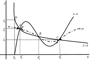
If the slope of forest resource demand curve is zero at $(\lambda, S)$ space, then $\frac{d \lambda}{d S}=-\frac{z_{S}}{z_{\lambda}}<0 ;$ the implicit supply curve slope can be greater than zero or less than zero. At $(\lambda, S)$ space of supply curve and demand curve there are at least two steady intersections and some unsteady intermediate state points, such as point B, steady state point $\mathrm{A}$ and point $\mathrm{C}: A\left(\lambda_{1}^{*}, S_{1}^{*}\right)$ is the higher price, lower stock; $C\left(\lambda_{3}^{*}, S_{3}^{*}\right)$ is a lower price, higher resource stock. Let's take the three intersections for examples to illustrate this relationship, as shown in Figure 1.
Figure 1. Implicit dynamic balance between supply and demand of forest resource
4.4.3 The steady-state forest resource degradation rules
As shown in Figure 1, the demand and supply curve on the left region of point A exhibits the demand of forest resource is greater than its supply, forest degradation is accelerating, even forest resource is exhausted on the left region of point D.
Rearrange (16), (18), (22), and obtain
$d_{S R}=g_{S R}-\delta$ (31)
where, $d_{S R}=\frac{d\left((1-\theta) G_{2}-X^{\prime}\right)}{d t} /\left[(1-\theta) G_{2}-X^{\prime}\right]$, denotes forest resource degradation rate in time direction; $g_{S R}=\frac{d\left(U_{3}+U_{1} G_{2}\right)}{d t} /$ $\left(U_{3}+U_{1} G_{2}\right)$ denotes the marginal utility growth rate in the direction of time related to forest resources stock.
Proposition 4 can be obtained from (31).
Proposition 4 long-term equilibrium state, the forest resources inventory $(S)$ by marginal utility rate related to forest resources inventory decisions together with the social discount rate. And degradation of forest resources; Where $d_{S R}=$ $\frac{d\left((1-\theta) G_{2}-X^{\prime}\right)}{d t} /\left[(1-\theta) G_{2}-X^{\prime}\right]$, denotes forest resource degradation rate in time direction; $g_{S R}=\frac{d\left(U_{3}+U_{1} G_{2}\right)}{d t} / U_{3}+$ $U_{1} G_{2}$ denotes the marginal utility growth rate in the direction of time related to forest resources stock.
Proposition 4 can be obtained from (31).
Proposition 4 In long-term equilibrium state, the forest resource stock $\left(S^{*}\right)$ is determined by the marginal utility growth rate related to the forest resource stock along with the social discount rate. If $g_{S R}>\delta$, forest resource degrades; if $g_{S R}<\delta$, forest resource is sustainable; if $g_{S R}=\delta$, the forest resource stock in the long-term equilibrium state is determined by $(1-\theta) \dot{G}_{2}=\dot{X}^{\prime}$.
As given by (21), trade measures make terms of trade $\left(P_{w}\right)$ improved or worsen, and affect the level of resource good export and manufactures import, then lead to the change of forest resource stock level. Analyze the relationship between forest resource stock level change and terms of trade, that is, $\frac{d S^{*}}{d P_{W}}$, then rewriting Eqns. (21), (29), and (30) yields
$U_{1}\left(G\left(N_{f}^{*}, S^{*}\right)-E_{f}^{*}\right)-U_{2}\left(F\left(N-N_{f}^{*}\right)+P_{w} E_{f}^{*}\right) P_{w}$$=0$ (32)
$X\left(S^{*}\right)-(1-\theta) G\left(N_{f}^{*}, S^{*}\right)=0$ (33)
$U_{1}\left(G\left(N_{f}^{*}, S^{*}\right)-E_{f}^{*}\right) G_{1}\left(N_{f}^{*}, S^{*}\right)-U_{2}\left(F\left(N-N_{f}^{*}\right)\right.$$\left.+P_{w} E_{f}^{*}\right) F^{\prime}\left(N-N_{f}^{*}\right)=0 \partial C_{f} / \partial S$$=G_{1} f_{1}+G_{2}-h_{1}>0$ (34)
Eq. (34) is the rewritten equation obtained from integrating (16), (17), (18), (20), and (22) to yield $U_{1} G_{1}-U_{2} F^{\prime}=$ 0subject to $\dot{U}_{1}=\dot{U}_{2}=0$.
Respectively take a derivative of endogenous variables $\left(N_{f}^{*}, S^{*}, E_{f}^{*}\right)$ and exogenous variables $\left(P_{w}, \theta\right)$ by the differential equation system composed of (32), (33), (34), and it can be represented as:
From negative Hessian matrix and Cramer's rule, it can be known as the follows:
$\left|\begin{array}{ccc}U_{11} G_{1}-U_{22} F^{\prime} P_{w} & U_{11} G_{2} & -U_{11}+U_{22} P_{w}^{2} \\ -(1-\theta) G_{1} & X^{\prime}-(1-\theta) G_{2} & 0 \\ U_{11} G_{1}^{2}+U_{1} G_{11}+U_{22} F^{\prime} F^{\prime}+U_{2} F^{\prime \prime} & U_{11} G_{1} G_{2}+U_{1} G_{12} & -U_{11} G_{1}-U_{22} P_{w} F^{\prime}\end{array}\right|$$\left|\begin{array}{l}d N_{f}^{*} \\ d S^{*} \\ d E_{f}^{*}\end{array}\right|$
$=\left|\begin{array}{cc}-U_{2}-U_{22} E_{f}^{*} P_{w} & 0 \\ 0 & G \\ -U_{22} E_{f}^{*} F^{\prime} & 0\end{array}\right|\left|\begin{array}{c}d P_{w} \\ d \theta\end{array}\right|$
As given by Eq. (21), if $F^{\prime}<P_{w} G_{1}$, then; it is given by (22) as $X^{\prime}-(1-\theta) G_{2}>0$.
If $U_{11}-U_{22} P_{w}^{2}>0$, integrating all symbols of values yields: $J_{1}<0$.
$\frac{d S^{*}}{d P_{w}}=\frac{(1-\theta) G_{1}}{-\left|J_{1}\right|}\left[\left(U_{2}+U_{22} E_{f}^{*} P_{w}\right)\left(U_{11} G_{1}+U_{22} P_{w} F^{\prime}\right)\right.$$\left.+U_{22} E_{f}^{*} F^{\prime}\left(U_{22} P_{w}-U_{11}\right)\right]$ (35)
$U_{22} E_{f}^{*} F^{\prime}\left(U_{22} P_{w}-U_{11}\right)>0 ; U_{11} G_{1}+U_{22} P_{w} F^{\prime}<0 ;$ when $\frac{U_{2}}{U_{22}}<-E_{f}^{*} P_{w}, U_{2}+U_{22} E_{f}^{*} P_{w}<0 ;$ then $\frac{d s^{*}}{d P_{w}}>0$.
Proposition 5 In the case of $\frac{U_{11}}{U_{22}}>P_{w}^{2}$, and $\frac{U_{2}}{U_{22}}<-E_{f}^{*} P_{w}$, if terms of trade is improved, forest resource stock increases and forest degradation slows down; if terms of trade is deteriorated, forest resource stock declines, and forest degradation is intensified.
Relax assumption 6, provided that the domestic forest resource export affects the international market price, how does forest resource stock change? Define export market force of the domestic forest resource as follows:
Because Because $\varepsilon=E_{f}^{\prime} P_{w} / E_{f}$, then $E_{f}=E_{f}\left(P_{w}\right), E_{f}^{\prime}<0, E_{f}^{\prime \prime}>0$.
Rewriting Eqns. (32), (34) yields
$U_{1}\left(G\left(N_{f}^{*}, S^{*}\right)-E_{f}^{*}\right)-U_{2}\left(F\left(N-N_{f}^{*}\right)+P_{w}(1\right.$$\left.\left.+\frac{1}{\varepsilon}\right) E_{f}^{*}\right) P_{w}\left(1+\frac{1}{\varepsilon}\right)=0$ (32')
$X\left(S^{*}\right)-(1-\theta) G\left(N_{f}^{*}, S^{*}\right)=0$ (33')
$U_{1}\left(G\left(N_{f}^{*}, S^{*}\right)-E_{f}^{*}\right) G_{1}\left(N_{f}^{*}, S^{*}\right)-U_{2}\left(F\left(N-N_{f}^{*}\right)\right.$$\left.+P_{w}\left(1+\frac{1}{\varepsilon}\right) E_{f}^{*}\right) F^{\prime}\left(N-N_{f}^{*}\right)=0$ (34')
$\left|\begin{array}{ccc}U_{11} G_{1}-U_{22} F^{\prime} P_{w} & U_{11} G_{2} & Y 1 \\ -(1-\theta) G_{1} & X^{\prime}-(1-\theta) G_{2} & 0 \\ U_{11} G_{1}^{2}+U_{1} G_{11}+U_{22} F^{\prime} F^{\prime}+U_{2} F^{\prime \prime} & U_{11} G_{1} G_{2}+U_{1} G_{12} & Y 2\end{array}\right|$$\left|\begin{array}{l}d N_{f}^{*} \\ d S^{*} \\ d P_{w}\end{array}\right|$
$=\left|\begin{array}{cc}-\left\{U_{22} P_{w} E_{f}^{*} P_{w}\left(1+\frac{1}{\varepsilon}\right)+U_{2} P_{w}\right\} & 0 \\ 0 & G \\ -U_{22} E_{f}^{*} P_{w} & 0\end{array}\right|$$\left|\begin{array}{r}d \frac{1}{\varepsilon} \\ d \theta\end{array}\right|$
$Y 1=\frac{d\left(32^{\prime}\right)}{d P_{w}}=-U_{11} E_{f}^{\prime *}-U_{22}\left(1+\frac{1}{\varepsilon}\right) E_{f}^{*}(1+\varepsilon) P_{w}\left(1+\frac{1}{\varepsilon}\right)-U_{2}\left(1+\frac{1}{\varepsilon}\right)<0$
$2=\frac{d\left(34^{\prime}\right)}{d P_{w}}=-U_{11} E_{f}^{\prime *}-U_{22}\left(1+\frac{1}{\varepsilon}\right) E_{f}^{*}(1+\varepsilon) F^{\prime}<0$
Differentiate $N_{f}^{*}, S^{*}, P_{w}, \frac{1}{\varepsilon}, \theta$ by differential system composed of (32'), (33'), (34') It is rewritten as follows.
From negative Hessian matrix and Cramer 's rule, it can be known as the follows:
$J_{2}=Y 1 \cdot\left\{(1-\theta) G_{1}\left(U_{11} G_{1} G_{2}+U_{1} G_{12}\right)-\left(X^{\prime}-(1\right.\right.$$\left.-\theta) G_{2}\right)\left(U_{11} G_{1}^{2}+U_{1} G_{11}+U_{22} F^{\prime} F^{\prime}\right.$$\left.\left.+U_{2} F^{\prime \prime}\right)\right\}+Y 2 \cdot\left\{\left(U_{11} G_{1}-U_{22} F^{\prime} P_{w}\right)\left(X^{\prime}\right.\right.$$\left.\left.-(1-\theta) G_{2}\right)+U_{11} G_{1} G_{2}(1-\theta)\right\}<0$ (36)
$\frac{d S^{*}}{d \frac{1}{\varepsilon}}=\frac{1}{-\left|J_{2}\right|}\left\{-Y 2 \cdot\left[U_{22} P_{w}^{2} E_{f}^{*}\left(1+\frac{1}{\varepsilon}\right)+U_{2} P_{w}\right]+Y 1 \cdot U_{22} P_{w} E_{f}^{*}\right\}$
$1 / \varepsilon<-\left(U_{22} E_{f}^{*}+U_{1}\right) / U_{22}, d S^{*} / d(1 / \varepsilon)>0$, then proposition 6 is obtained.
Proposition 6 when condition $1 / \varepsilon<-\left(U_{22} E_{f}^{*}+U_{1}\right) /$ $U_{22}$ is satisfied, if market force is enhanced, the long-term forest resource stock increases, then forest degradation is improved; if Market forces is weakened, forest resource stock decreases, forest degrades. When Condition $1 / \varepsilon<$ $-\left(U_{22} E_{f}^{*}+U_{1}\right) / U_{22}$ is not satisfied, the forest resource stock may increase, decrease or be in other cases.
Relax hypothesis 8, if there is foreign debt or obligatory right, then there is a dynamic equation of foreign obligatory right:
$\dot{D}=P_{w} E_{f}-I_{i}+r D$ (37)
$D>0$ denotes foreign obligatory right (assets); $D<$ 0 denotes foreign debt (debt); $\mathrm{r}$ is the world interest rate. Refer to the literature of Barbier and Rauscher [13]; Kahn and McDonald [8]; Barbier and Rauscher [13] for other dynamic equation of foreign debt.
Add the dynamic condition given in (37), then rewrite the current value Hamilton function in section 4.1 as the following:
$\begin{aligned} H=U\left(C_{f}, C_{i}, S\right) &+\lambda\left(X(S)-(1-\theta) G\left(N_{f}, S\right)\right) \\ &+\rho\left(P_{w} E_{f}-I_{i}+r D\right) \end{aligned}$
$\rho$ is a covariate of foreign debt or obligatory right shadow price. Assume that there is an internal solution, and the following conditions can be obtained from Pontryagin maximum principle:
$U_{1}=b_{1}=P_{w} \rho$ (38)
$U_{2}=b_{2}=\rho$ (39)
$\dot{\lambda}=\lambda\left(\delta-X^{\prime}+(1-\theta) G_{2}\right)-b_{1} G_{2}-U_{3}$ (40)
$\dot{\rho}=(\delta-r) \rho$ (41)
For the notation of Eqns. (38), (39), and (40), see the above mentioned illustrations; Eq. (40) denotes the change rate of foreign asset price is determined by the opportunity cost $\delta-$ rof holding the asset. Equations from (38) to (41) imply the optimal path relationship between $U_{1}, U_{2}, U_{3}, \lambda, \rho$, namely,
$\delta-X^{\prime}=r-X^{\prime}=\frac{(1-\theta)\left(U_{2} G_{2} F^{\prime}+U_{3} G_{1}\right)}{U_{1} G_{1}-U_{2} F^{\prime}}$ (42)
$\dot{S}=\frac{\left(r-X^{\prime}\right)(\delta-r)}{C+X^{\prime \prime}}$ (43)
$(1-\theta)\left\{U_{2} F^{\prime} G_{22}\left(U_{1} G_{1}-1\right)\right.$$\quad+U_{33} G_{1}\left(G_{1} U_{1}-U_{2} F^{\prime}\right)$
$C=\frac{\left.-U_{2} U_{3} F^{\prime} G_{12}-U_{1} U_{2} F^{\prime} G_{2} G_{12}\right\}}{\left(U_{1} G_{1}-U_{2} F^{\prime}\right)^{2}}$
$G_{1} U_{1}-1>0, G_{1} U_{1}-U_{2} F^{\prime}>0$, given by(21) along with other conditions (see hypothesis in the paper) can yield $C<0$.
Eq. (42) is the social efficiency condition, which denotes the optimal yield of forest resource stock $X^{\prime}+\frac{(1-\theta)\left(U_{2} G_{2} F^{\prime}+U_{3} G_{1}\right)}{U_{1} G_{1}-U_{2} F^{\prime}}$ equals to foreign assets yield $r$; Eq. (43) denotes the optimal growth path of resource stock. If the opportunity cost of holding forest resource stock is negative, forest resource stock increases; if the opportunity cost of holding forest resource stock is positive, forest degrades. Summarize the implied relation to get proposition 7.
Proposition 7 Provided that the transnational capital market and forest resource stock satisfy the positive external conditions $\left(U_{3}>0\right)$, forest resource stock will never be extinguished, and will be sustainable. The long-term equilibrium forest resource stock is determined by $\delta=r=$ $X^{\prime}+\frac{(1-\theta)\left(U_{2} G_{2} F^{\prime}+U_{3} G_{1}\right)}{U_{1} G_{1}-U_{2} F^{\prime}}$
The paper studies the association of foreign trade, market force, foreign debts or obligary right with forest resource stock to find some important features.
Firstly, provided that the forest resource stock satisfies the positive external conditions and there is forest restoration department, The long-term equilibrium forest resource stock is higher than the equilibrium level of forest resource stock shown in the literature of McRAE [12], Barbier and Rauscher [21] and Chen [22, 23]. If the social shadow price of forest resource stock is higher than $\lambda_{1}^{*}$ due to some factor, then the forest resource stock demand exceeds supply, and thus directly leads to the decrease, degradation, and even exhaustion of the forest resource stock. The conditions of Pontryagin maximum principle show that its effects work from the labor allocation used in resource sector $\left(N_{f}^{*}\right)$.
Secondly, the restriction to import and export of forest resource good will lead to the improvement or deterioration of terms of trade, thereby influence the dynamics of forest resource stock. If $\frac{U_{11}}{U_{22}}>P_{w}^{2}$, and $\frac{U_{2}}{U_{22}}<-E_{f}^{*} P_{w}$ exists, the forest resource stock and terms of trade change in the same direction- terms of trade deteriorates, forest resource stock declines, and forest degrades.
Thirdly, when the forest resource good exporting countries have impact on world market of resource good, if $\frac{1}{\varepsilon}<$ $-\left(\frac{U_{22} E_{f}^{*}+U_{1}}{U_{22}}\right)$ is satisfied, forest resource dynamic and market force change in the same direction, but if the condition is not satisfied, the dynamic change direction of forest resource stock is not clear.
Finally, in the case of relaxing trade balance condition, the trade deficit (liabilities) or surplus (assets), and considering transnational capital market, the forest resource stock will not be extinguished, and will be sustainable, but the long-term equilibrium forest resource stock is determined by $\delta=r=$ $X^{\prime}+\left[(1-\theta)\left(U_{2} G_{2} F^{\prime}+U_{3} G_{1}\right)\right] /\left(U_{1} G_{1}-U_{2} F^{\prime}\right)$.
This work is supported by the Evaluation Committee of Social Science Achievements of Hunan Province (Grant No.: XSP22YBC334).
[1] Forest Resources Assessment 2010. http://www.fao.org/docrep/013/i1757e/i1757e.pdf,2017-05-29.
[2] WRI. (2017). Forests: sustaining forests for people and planet. http://www.wri.org/our-work/topics/forests,2017-05-29.
[3] Shimamoto, M., Ubukata, F., Seki, Y. (2004). Forest sustainability and the free trade of forest products: Cases from Southeast Asia. Ecological Economics, 50(1-2): 23-34. http://dx.doi.org/10.1016/j.ecolecon.2004.02.004
[4] Jinji, N. (2006). International trade and terrestrial open‐access renewable resources in a small open economy. Canadian Journal of Economics/Revue canadienne d'économique, 39(3): 790-808. http://dx.doi.org/10.1111/j.1540-5982.2006.00370.x
[5] Tsurumi, T., Managi, S. (2014). The effect of trade openness on deforestation: empirical analysis for 142 countries. Environmental Economics and Policy Studies, 16(4): 305-324. http://dx.doi.org/10.1007/s10018-012-0051-5
[6] Shimamoto, M. (2008). Forest sustainability and trade policies. Ecological Economics, 66(4): 605-614. http://dx.doi.org/10.1016/j.ecolecon.2007.10.019
[7] Capistrano, A.D., Kiker, C.F. (1995). Macro-scale economic influences on tropical forest depletion. Ecological Economics, 14(1): 21-29. http://dx.doi.org/10.1016/0921-8009(95)00008-W
[8] Kahn, J.R., McDonald, J.A. (1995). Third-world debt and tropical deforestation. Ecological Economics, 12(2): 107-123. http://dx.doi.org/10.1016/0921-8009(94)00024-P
[9] Arcand, J.L., Guillaumont, P., Jeanneney, S.G. (2008). Deforestation and the real exchange rate. Journal of Development Economics, 86(2): 242-262. http://dx.doi.org/10.1016/j.jdeveco.2007.02.004
[10] Richards, P.D., Myers, R.J., Swinton, S.M., Walker, R.T. (2012). Exchange rates, soybean supply response, and deforestation in South America. Global environmental change, 22(2): 454-462. http://dx.doi.org/10.1016/j.gloenvcha.2012.01.004
[11] Kemp, M.C., Suzuki, H. (1975). International trade with a wasting but possibly replenishable resource. International Economic Review, 16(3): 712-732. http://dx.doi.org/10.2307/2526005
[12] McRae, J.J. (1978). Optimal and competitive use of replenishable natural resources by open economies. Journal of International Economics, 8(1): 29-54. http://dx.doi.org/10.1016/0022-1996(78)90037-5
[13] Barbier, E.B., Rauscher, M. (1994). Trade, tropical deforestation and policy interventions. In Trade, Innovation, Environment. http://dx.doi.org/10.1007/BF00691933
[14] Plourde, C.G. (1971). Exploitation of common-property replenishable natural resources. Economic Inquiry, 9(3): 256-266. http://dx.doi.org/10.1111/j.1465-7295.1971.tb01640.x
[15] Vanek, J. (1963). The natural resources content of United States foreign trade. MIT Press, [Massachusetts institute of technology].
[16] Faustmann, M. (1968). On the determination of the value which forest lands and immature stands pose for forestry, 1849, in: M. Gane, ed., Martin Faustmann and the evolution of discounted cash flow, Oxford Institute.
[17] Clarke, H.R., Shrestha, R.M. (1986). Long run equilibrium properties of renewable resource management models. Resources and energy, 8(3): 279-308. http://dx.doi.org/10.1016/0165-0572(86)90006-X
[18] Clark, C.W., Clarke, F.H., Munro, G.R. (1979). The optimal exploitation of renewable resource stocks: problems of irreversible investment. Econometrica: Journal of the Econometric Society, 47(1): 25-47. http://dx.doi.org/10.2307/1912344
[19] Burghes, D.N. (1980). Renewable resource depletion: the conservation problem. International Journal of Mathematical Educational in Science and Technology, 11(2): 221-229. http://dx.doi.org/10.1080/0020739800110213
[20] Clark, C.W. (1979). Mathematical models in the economics of renewable resources. Siam Review, 21(1): 81-99. http://dx.doi.org/10.1137/1021006
[21] Chen, H. (2017). International trade, property maintenance intensity and renewable resources sustainability. Advances in Modelling and Analysis A, 54(1): 1-20. https://doi.org/10.18280/ama_a.540101
[22] Chen, H. (2018). International trade, urbanization and forest resource dynamics. Journal of Interdisciplinary Mathematics, 21(4): 859-867. https://doi.org/10.1080/09720502.2018.1475066
[23] Chen, H. (2019). Connotation of forest degradation and the measure of forest degradation in China. Taru Journal of Organizational Behavior & Analytics, 1(1): 15-28. https://doi.org/10.47974/TJOBA.005.2019.v01i01