Eali Stephen Neal Joshua![]() | Debnath Bhattacharyya
| Debnath Bhattacharyya![]() | Thirupathi Rao Nakka
| Thirupathi Rao Nakka![]() | Yung-Cheol Byun*
| Yung-Cheol Byun*![]()
© 2023 IIETA. This article is published by IIETA and is licensed under the CC BY 4.0 license (http://creativecommons.org/licenses/by/4.0/).
OPEN ACCESS
Lung cancer is the leading cause of mortality worldwide, affecting both men and women equally. Identifying and treating these nodules when they are still tiny may increase their chances of survival significantly. However, due to the large amount of data generated by this CT scanner, manual segmentation and interpretation takes a long time and is quite challenging to do on your own. When a radiologist focuses on the patient's body, it increases the strain on the radiologist, and the likelihood of missing pathological information, such as abnormalities, is also increased. One of the primary objectives of this project is to develop computer-assisted diagnosis and detection of lung cancer. It also intends to make it easier for radiologists to identify and diagnose lung cancer more rapidly and accurately. Based on a unique picture feature, the proposed strategy k into consideration the spatial interaction of voxels that were next to one another. Using the U-NET+Three parameter logistic distribution-based technique, we were able to replicate the situation. According to the researchers, the proposed technique method DSC of 97.3%, a sensitivity of 96.5%, and a specificity of 94.1% when tested on the LuNa-16 dataset. At long last, this research investigates how diverse lung segmentation, juxta pleural nodule inclusion, and pulmonary nodule segmentation approaches may be applied to create CAD systems. Other objectives include making it possible to conduct research into lung segmentation and automated pulmonary nodule segmentation while also improving the power and effectiveness of computer-assisted diagnosis of lung cancer, which relies on correct pulmonary nodule segmentation to be successful.
lung cancer, LuNa-16, LIDC/IDRI, CAD systems, segmentation, deep learning, CT scans, U-NET
Lung cancer is the leading cause of mortality in the world, affecting both men and women equally. According to the American Cancer Society, 222,500 new instances of lung cancer [1, 2] were diagnosed in 2017 [3], and 155,870 individuals died as a result of the disease. The survival rate for colon cancer is 65.4%, whereas breast cancer has a survival rate of 90.35%, and prostate cancer has a survival rate of 99.6%, which is much lower than the overall survival rate of 65.4% [4]. It's possible that a lung nodule is an indication of lung cancer. Only 16% of cases are discovered in the early stages. If these nodules are discovered while they are still in their original location, the odds of survival increase from 10% to 65-70%.
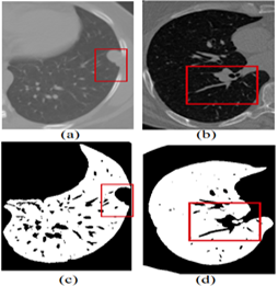
Lung cancer is detected and treated with the use of imaging methods such as multidetector X-ray computed tomography (MDCT) [5]. If you have a CT scanning today, you will get a large amount of information. Performing all of this data segmentation and analysis by hand is difficult and time-consuming. It makes the work of the radiologist more complicated and time-consuming. Glancing at a large number of images can increase the likelihood of missing essential clinical criteria, such as abnormalities, was shown in the Figure 1.
Figure 1. Showing the limitations of the normal image-based segmentation
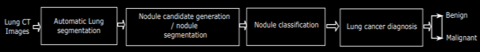
In order to address this issue, computer-assisted diagnosis (CADx) [6] and computer-assisted detection (CADe) have been investigated as potential methods of assisting radiologists with CT scans while also improving their diagnostic accuracy. For the last two decades, researchers from all around the globe have been focusing their efforts on strategies to increase the accuracy of lung nodule detection. The four major components of the CAD/CADe system are shown in Figure 2. 1) The lungs are immediately divided into two halves. 2) Selection of nodule candidates or division of nodules is two examples of nodule division. 3) Nodules and the many forms of nodules. 4) It was discovered that the patient had lung cancer. Auto lung segmentation is the most critical step in the pre-processing stage of the CAD system. This is done prior to the discovery or identification of lung nodules.
Figure 2. Showing the basic block diagram of the CADx systems
For lung segmentation, there are two primary goals: to reduce the amount of time it takes to do the calculation and to ensure that a search only goes to the lung parenchyma by making sure the boundaries are extremely well defined. This is due in part to the fact that the radio density of the juxta pleural nodule is the same as that of the chest region, which means that segmentation does not always pick it up on the scan. There have been several reports of various methods [7] of dividing the lung, but only a handful of them have been shown to involve juxta pleural nodules. During the second stage of the construction process, basic image processing methods are used to identify a variety of nodules in the lung area that have been successfully healed. The final step makes use of machine learning to determine which objects include nodules and which ones do not contain nodules (e.g., segments of airways, arteries, or other non-cancerous lesions).
In order to examine the lung parenchyma, high-resolution computer tomography is used (HRCT). A three-dimensional depiction of the human thorax is included, as well as high spatial and temporal resolutions in both space and time. Apart from the fact that it has a three-dimensional form, it provides excellent contrast resolution for pulmonary structures and surrounding tissue.
CT imaging is utilized to examine the parenchyma, airways, and mechanics of the diaphragm in the lungs. It turns out that when CT scanners improve in quality, the frequency of volumetric lung studies increases as well. Manual segmentation of a large number of CT slices [8] becomes impossible as a result of this. Consequently, automated lung segmentation is being utilized to distinguish the lungs from the rest of the body.
The Major Contributions of the proposed research work are as follows:
·To develop the algorithm for lung Segmentation and lobe volume quantification.
·To develop automatic segmentation of lungs field with various abnormal patterns attached to lung boundary such as excavated mass, pleural nodule, etc.
·To design the lung segmentation algorithm for the inclusion of juxta pleural nodules and pulmonary vessels.
·To design the algorithm for the segmentation of various types and shapes of pulmonary nodules.
Convolutional neural networks are used in the creation of UNET [9]. Despite the fact that this network has just 23 layers, it performs well. Although it is not as difficult as networks with hundreds of layers, it nevertheless requires a significant amount of effort. Down- and up-sampling is used extensively in a single network environment. During the down-sampling step, you may use convolutional and pooling layers to identify characteristics in the picture that you want to maintain and keep in the final image.
Deconvolution is used to make the map of features more visible by removing some of the details [10]. Depending on where you reside, this is referred to as a decoder or an encoder. If you utilize a convolution or pooling layer, you will obtain feature maps that include varying amounts of information from the images with which they are merged, depending on the layer you select. They each include a varied quantity of information about themselves.
Following upsampling, a technique known as deconvolution is performed to increase the size of the feature map. In the next step, the original feature map is blended with a down-sampled feature map. This is done in order to recover the abstract data that has been lost and to enhance network segmentation and segmentation accuracy.
On a CT image of the lungs, we can observe how the UNET network learns about nodules via convolution and pooling of information. This implies that a significant amount of spatial information is lost. A significant amount of information regarding how events will unfold is lost as a consequence of sample reductions. People who create up sampled photos do not achieve the same clarity as those who create original images.
When all of the aforementioned problems are taken into consideration, it is critical to establish temporary UNET networks in order to improve the situation even more. Why there hasn’t been enough study on how to discover lung cancer nodules that have been divided into segments is explained in Table 1.
Researchers [11-20] used an identical data set, but the model's robustness was degraded. Because the U-NET could not be utilized with new data types, the IOU intersection and dice co-efficient index accuracy were unavailable. This concept enhances the efficiency of fully linked and multiscale conversion systems. The previous models had the following main flaws:
Gradient’s descent fades away as one moves farther from the network's error computation and training data output. Weakly evolving intermediate stratum models may opt to skip using abstract layers altogether. The Following research questions were not addressed properly. They are listed as follows:
·Why If the object of interest is not a typical shape or is outside the image, the U-Net architecture cannot extract information from it.
·It seems that the suggested DB-NET Models' benefits outweigh any disadvantages produced by their intermediary layers' fewer steep slopes. These experiments found that DB-NETs outperform other designs at recognizing small items in pictures. Modeling models that aren't similar or include new technology is straightforward and quick.
·When making technical decisions, all model versions must be given the same weight. This is especially true when updating or improving current models. Paying attention to the specifics while judging a model's technological design is crucial. In medicine, biomedical imaging may reveal heterochromatin concentrations and synapses in the brain, among other things.
·To correctly distribute light, orientation, and components, an algorithm may need to recognize the same item again on a very small scale. Convolutional networks may be able to gain these traits without giving up any of their existing knowledge. However, when compared to other previously evaluated models, DB-NET outperformed them with more data. The LUNA16 benchmark dataset gave us a wide range of data to examine our model.
Table 1. Showing the literature survey and gap in lung cancer classification
|
Ref |
Research Objective |
Approach |
Segmentation Technique |
DSC (%) |
Outcome and Result |
Research Gap |
Dataset |
Split (%) |
|
[11] |
Segmentation Method to find out the Benign and Malignant Nodule |
Deep Learning Approach- CNN-based Segmentation |
CNN with Overlapped subdiaphragmatic Space |
92.23% |
To determine how well the model performed, we looked at its sensitivity and the average number of false positives per picture in a separate collection of photos from the original set (mFPI). The training set had 629 radiographs, whereas the test set contained 151 radiographs. The training set had 652 nodules and 159 masses, whereas the test set contained 151 nodules and 159 masses. |
The Model failed to produce accurate results on minimal dataset. |
LIDC-IDRI/ LUNA-16 |
70:30 |
|
[12] |
Segmentation of the Lung CT scan images |
3D-Segmentation |
Deep Supervision architecture |
84.75% |
This work aims to investigate lung tumour segmentation utilising a two-dimensional DWT and a Deeply Supervised MultiResUNet model, both of which have been developed recently. It is necessary to utilise the LOTUS dataset, which contains 31,247 training samples and 4458 testing samples. In addition, a Deeply Supervised MultiResUNet model is used. A combination of deep supervision in model design with DWT results in a more extensive textural analysis that takes into consideration information from nearby CT slices, which improves the results. |
Golden Standards of the Algorithm was not gaining the trust |
LIDC-IDRI/ LUNA-16 |
60:40 |
|
[13] |
Lung Cancer Segmentation on Low-Dose Ct scans with improvised Classifier. |
Deep-learning Model CT2Rep |
Segmented related Nodule Feature on Low Dose CT scans |
92.29% |
Following training, the model continues to improve its performance as a result of input from those who use it. Lung cancer lesion segmentation on PET/CT images is accomplished using FSL, and we use a U-Net architecture to modify the weights of the models. An online supervised learning approach is created as a consequence of this, which allows for dynamic model weight adjustments. |
The Coordinates if the images were misplaced and not accurately done. |
LIDC-IDRI/ LUNA-16 |
70:30 |
|
[14] |
Lung Lesion benign Tumour Segmentation with improvised U-NET |
CADe for increased performance of Lung Cancer Segmentation with FSL Model |
Two- Parameter Logistic Distribution with Improvised U-NET architecture |
92.68% |
One of the objectives of this research was to apply deep learning to develop a system that could be used to correctly and reliably segment lung nodule regions in three dimensions. This research demonstrated how to employ a three-dimensional fully connected convolutional network with residual unit structures and a novel loss function in conjunction with a three-dimensional convolutional network. |
The main disadvantages of this model are Heavyweight architecture. |
LIDC-IDRI/ LUNA-16 |
60:40 |
|
[15] |
3D CT scan with improvised Fully connected CNN |
3D Convolutional Neural Network with Annotated images. |
Two- Parameter Logistic Distribution with Fill Connected CNN architecture |
96.4% |
When a person has lung cancer, he or she may have a variety of additional respiratory disorders, each with its own set of CT imaging results. A deep learning model with two distinct structures: a U-Net and a ResNet34 — is being developed as part of this project's efforts. |
The standard deviation and mean accuracy of the model were very low. |
LIDC-IDRI/ LUNA-16 |
70:30 |
|
[16] |
Lung Cancer Segmentation with Cross – Cohort |
Residual U-NET with annotated images |
Two- Parameter Logistic Distribution with a Residual U-NET approach. |
96.58% |
In order to create the images for the deep learning model, the researchers employed a number of image preparation approaches. Image resampling, intensity normalization, 3D nodular patch cutting, and data augmentation were some of the techniques used. The residual network and the atrous spatial pyramid pooling module, as well as a 3D attentional cascaded residual network, were then used to construct the final model (ACRU-Net). |
This work failed to explain the hidden features in the Low Dose CT scan images. |
LIDC-IDRI/ LUNA-16 |
70:30 |
|
[17] |
Lung Cancer Volumetric Segmentation |
Residual U-NET with random field |
Two- Parameter Logistic Distribution with a cascaded Residual U-NET approach. |
95.36% |
Deep learning networks are utilized in this approach of finding objects via deep learning. They beat the best segmentation networks, such as the U-net network, in terms of overall performance. |
The Model Prediction and AUC curves were not golden standards. |
LIDC-IDRI/ LUNA-16 |
70:30 |
|
[18] |
Lung Cancer Segmentation with the CNN |
Residual and Separable CNN with Shallow layers |
Two- Parameter Logistic Distribution with CNN- Residual Separable Network approach. |
94.56% |
This deep learning technique uses deep learning networks to detect things. Ensemble methods, maximum intensity projection-based preprocessing, and two novel deep learning networks are included. In Deep Residual Separable Convolutional Neural Networks 1 and 2, what occurred was: A choice was made. Overall, they outperformed the best segmentation networks like U-net. |
The model was shown more loss when the high-dose CT scan images were given as output |
LIDC-IDRI/ LUNA-16 |
70:30 |
|
[19] |
Lung Cancer Segmentation with the 4D CT scans |
Multiplanar U-NET for high-dose CT scan images. |
Motion Mask Segmentation using Two Parameter Segmentation |
91.56% |
This study demonstrates that it is feasible to tackle this issue using a lightweight deep-learning technique that can be implemented on a single machine and does not need the collection of a large amount of additional data or the development of complex models. |
Diversity in training data is missing. |
LIDC-IDRI/ LUNA-16 |
70:30 |
|
[20] |
Lung Cancer Segmentation on 4D CT scans |
Motion Neural Network with two parameters |
R-CNN with the local motion CT scans |
96.89% |
As part of the planned deep learning architecture, it is used. In this particular instance, the motion region convolutional neural network is used (R-CNN). |
Annotated images with few data augmentation results in the diversity of the classifier. |
LIDC-IDRI/ LUNA-16 |
70:30 |
3.1 Three logistic distribution
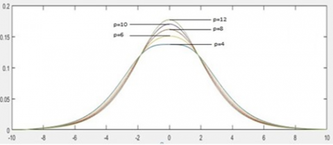
An effective methodology for estimating the parameters of mixture distribution is utilizing the Expectation-Maximization algorithm given by Turner et al. [21]. The efficiency of the EM algorithm depends on the initial values of the parameters and the number of mixture components in the model. Yang et al. [22] had utilized the K-means algorithm for obtaining initial values of the model parameters. the performance comparison has been taken by the k-means algorithm and hierarchical clustering algorithm; it is required to assign an initial value to the number of image regions. To overcome this disadvantage the hierarchal clustering algorithm is used for obtaining the number of components in the mixture model and initializing the model parameters. In this paper it is assumed that the pixel intensities of the image regions follow a logistic type distribution based on three parameters as a result, the whole image is considered by a k-component mixture with logistic type distribution which was based on three parameters.
The probability distribution function (P.D.F) of the current model is given by:
$f\left(z, \beta, \sigma^2\right)=\frac{\left[\frac{3}{\left(3 p+\pi^2\right)} \ \right]\left[p+\left(\frac{z-\beta}{\sigma} \; \right)^2\right] e^{-\left(\frac{z-\beta}{\sigma}\right)}}{\sigma\left[1+e^{-\left(\frac{z-\beta}{\sigma}\right)} \ \right]^2}$ (1)
where, -∞<z<∞, -∞<β<∞, p≥4.
The frequency curves associated with logistic type distribution for three parameters are shown in the Figure 3.
Figure 3. Three parameter-based frequency curves of logistic type distribution
The distribution function of the current model with β and the model is symmetric as:
$F(Z)=\frac{3 e^{-\left(\frac{z-\beta}{\sigma}\right)}}{\sigma^2\left(12+\pi^2\right)} \frac{\left[\left[4+\left(\frac{z-\beta}{\sigma}\right)^2\right]\left[2\left(\frac{z-\beta}{\sigma}\right)-1\right] e^{-\left(\frac{z-\beta}{\sigma}\right)^2}-\left[\left(\frac{z-\beta}{\sigma}\right)-1\right]^2\right]}{\left[1+e^{-\left(\frac{z-\beta}{\sigma}\right)^2}\right]^2}$ (2)
The probability density function (p.d.f) of the pixel intensities is of the form:
$f\left(z, \beta, \sigma^2, x\right)=\frac{\left[\frac{3}{\left(3 x+\pi^2\right)} \; \right]\left[x+\left(\frac{z-\beta}{\sigma}\right)^2\right] e^{-\left(\frac{z-\beta}{\sigma}\right)}}{\sigma\left[1+e^{-\left(\frac{z-\beta}{\sigma}\right)} \; \right]^2}$ (3)
where, -∞<z<∞, -∞<β<∞, x≥4, σ2>0.
3.1.1 Using the EM algorithm, the estimation of model parameters
For Expectation-Maximization (EM) algorithm, the updated equations of the model parameters the estimation error after calculation was 0.001. It’s an unbiased estimation.
Three parameter logistic type distribution:
$\log L(\theta)=\sum_{S=1}^N \log \left[\sum_{i=1}^m \alpha_i \frac{\left[\frac{3}{\left(3 p+\pi^2\right)} \; \right]\left[p+\left(\frac{x_s-\mu_i}{\sigma_i}\right)^2\right] e^{-\left(\frac{x_s-\mu_i}{\sigma_i}\right)}}{\sigma_i\left[1+e^{-\left(\frac{x_s-\mu_i}{\sigma_i}\right)} \; \right]^2} \, \, \, \right]$ (4)
The process of estimating the likelihood function on sample observations is considered the first step of the EM algorithm and is obtained as:
E-STEP:
In the expectation (E) step, the expectation value of log L(θ) concerning the initial parameter vector θ(0) is:
$Q\left(\theta, \theta^{(0)}\right)=E_{\theta^{(0)}}[\log L(\theta) / \bar{x}]$ (5)
This implies:
$\log L(\theta)=\sum_{S=1}^N \log \left(\sum_{i=1}^k \alpha^{(l)}{ }_i f_i\left(x_s, \theta^{(l)}\right)\right)$ (6)
The provisional likelihood which goes to region ‘k’ is:
$P_k\left(x_s, \theta^{(l)}\right)=\left[\frac{\alpha_k^{(l)} f_k\left(x_s, \theta^{(l)}\right)}{p_i\left(x_s, \theta^{(l)}\right)}\right]$ (7)
$p_k\left(x_s, \theta^{(l)}\right)=\left[\frac{\alpha_k^{(l)} f_k\left(x_s, \theta^{(l)}\right)}{\sum_{i=1}^k \alpha_i^{(l)} f_i\left(x_s, \theta^{(l)}\right)}\right]$ (8)
Therefore, for three parameter logistic type distribution:
$f_i\left(x_s, \theta^{(l)}\right)=\frac{\left[\frac{3}{\left(3 p+\pi^2\right)} \; \right]\left[p+\left(\frac{x_s-\mu_i^{(l)}}{\sigma^{(l)}}\right)^2\right] e^{-\left(\frac{x_s-\mu_i(l)}{\sigma_i(l)}\right)}}{\sigma_i^{(l)}\left[1+e^{-\left(\frac{x_s-\mu_i^{(l)}}{\sigma_i(l)}\right)}\right]^2}$ (9)
M-STEP:
To get the model parameters estimation, one should increase Q(θ, θ(l)) such that $\sum \alpha_i=1$. This estimation could be achieved by using the first order Lagrange type function:
$F=\left[E\left(\log L\left(\theta^{(l)}\right)\right)+\beta\left(1-\sum_{i=1}^k \alpha_i^{(l)}\right)\right]$ (10)
The updated equations of αi:
To find the expression for αi, we solve the following equation:
$\begin{gathered}\frac{\partial F}{\partial \alpha_i}=0 \\ \sum_{i=1}^N \frac{1}{\alpha_i} P_i\left(x_s, \theta^{(l)}\right)+\beta=0\end{gathered}$ (11)
After adding on both sides, β=-N.
Therefore,
$\alpha_i=\frac{1}{N} \sum_{s=1}^N P_i\left(x_s, \theta^{(l)}\right)$ (12)
The updated equations of αi for (l+1)th iteration is:
$\alpha_i^{(l+1)}=\frac{1}{N} \sum_{s=1}^N P_i\left(x_s, \theta^{(l)}\right)$ (13)
This implies:
$\alpha_l^{(l+1)}=\frac{1}{N} \sum_{s=1}^N\left[\frac{\alpha_l^{(l)} f_l\left(x_s, \theta^{(l)}\right)}{\sum_{i=1}^k \alpha_i^{(l)} f_i\left(x_s, \theta^{(l)}\right)}\right]$ (14)
The updated equations of μi:
For Two parameter logistic type distribution:
By applying the derivative with respect to μi, we have
$\frac{\partial}{\partial \beta_i}\left[\sum_{s=1}^N \sum_{i=1}^K P_i\left(x_{s,}, \theta^l\right) \log \alpha_i \frac{\left.\left[\frac{3}{12+\pi^2} \; \right]\left[4+\left(\frac{x_s-\beta_i}{\sigma_i}\right)^2\right] e^{-\left(\frac{x_s-\beta_i}{\sigma_i}\right)} \; \right]}{\sigma_i\left[1+e^{-\left(\frac{x_s-\beta_i}{\sigma_i}\right) \, \, ^2}\right]}\right]=0$ (15)
$\frac{\partial}{\partial \beta_i}\left[\sum_{s=1}^N \sum_{i=1}^K P_i\left(z_{s .}, \theta^l\right) \log \alpha_i \frac{\left.\left[\frac{3}{12+\pi^2} \; \right]\left[4+\left(\frac{z_s-\beta_i}{\sigma_i}\right)^2\right] e^{-\left(\frac{z_s-\beta_i}{\sigma_i} \; \right)} \; \,\right]}{\sigma_i\left[1+e^{-\left(\frac{z_s-\beta_i}{\sigma_i}\right) \;^2}\right]}\right]=0$ (16)
This implies:
$\sum_{s=1}^N P_i\left(x_s, \theta^l\right)\left[\left[\frac{2\left(\frac{z_s-\beta_i}{\sigma_i}\right)\left(-\frac{1}{\sigma_i}\right)}{\left[4+\left(\frac{z_S-\beta_i}{\sigma_i}\right)^2\right]}\right]+\left[\frac{1}{\sigma_i}\right]-\left[\frac{e^{-\left(\frac{z_s-\beta_i}{\sigma_i}\right) \, \, ^2} 2}{\sigma_i\left(1+e^{-\left(\frac{z_s-\beta_i}{\sigma_i}\right)^2} \; \, \right)} \right]=0\right.$ (17)
Since μi appears in only one region, i=1, 2, 3, ……, k. (regions).
For Three parameter logistic type distribution:
$\frac{\partial}{\partial \beta_i}\left[\sum_{s=1}^N \sum_{i=1}^K P_i\left(z_{s .}, \theta^l\right) \log \left[\alpha_i \frac{\left[\frac{3}{3 p+\pi^2} \, \, \right]\left[p+\left(\frac{z_s-\beta_i}{\sigma_i}\right)^2\right] e^{-\left(\frac{z_s-\beta_i}{\sigma_i}\right)}}{\sigma_i\left[1+e^{-\left(\frac{z_s-\beta_i}{\sigma_i} \; \right)} \; \right]^2} \; \; \right]\right]=0$ (18)
Finally:
For Three parameter logistic type distribution:
$\mu_i^{(l+1)}=\frac{\sum_{s=1}^n \frac{P_i\left(z, \theta^{(l)}\right)\left(2 y_s\right)}{\left(\sigma_i^2\right)^{(l)}\left[p+\left(\frac{z_s-\beta_i^{(l)}}{\sigma_i^{(l)}}\right)^2\right]}-\sum_{s=1}^n \frac{P_i\left(z_{s.}, \theta^{(l)}\right)}{\sigma_i^{(l)}}+\sum_{s=1}^n \frac{2 P_i\left(z_{s.}, \theta^{(l)}\right)}{\sigma_i^{(l)}\left[1+e^{\left.\left(\frac{z_s-\beta_i^{(l)}}{\sigma_i^{(l)}}\right)\right]}\right]}}{2 \sum_{s=1}^n \frac{P_i\left(z_{s.}, \theta^{(l)}\right)}{\left(\sigma_i^2\right)^{(l)}\left[p+\left(\frac{z_s-\beta_i^{(l)}}{\sigma_i^{(l)}}\right)^2\right]}}$ (19)
The updated equation of $\sigma_i^2$:
For updating $\sigma_i^2$ we differentiate $Q\left(\theta, \theta^{(l)}\right)$,
That is $\frac{\partial}{\partial \sigma^2}\left(Q\left(\theta, \theta^{(l)}\right)\right)=0$
This implies $E\left[\frac{\partial}{\partial \sigma^2}\left(\log L\left(\theta, \theta^{(l)}\right)\right)\right]=0$
$\frac{\partial}{\partial \sigma_i^2}\left[\sum_{s=1}^N \sum_{i=1}^K P_i\left(x_{s,}, \theta^l\right) \log \alpha_i \frac{\left[\frac{3}{12+\pi^2} \; \right]\left[4+\left(\frac{z_s-\beta_i}{\sigma_i}\right)^2\right] e^{-\left(\frac{z-\beta_i}{\sigma_i}\right)}}{\sigma_i\left[1+e^{-\left(\frac{z_s-\beta_i}{\sigma_i}\right) \; ^2} \; \right]} \; \; \right]=0$ (20)
This implies:
$\sum_{s=1}^N p_i\left(z s, \theta^{(l)}\right)\left[\frac{-\left(z_s-\beta_i\right)^2 \sigma_i^2}{\sigma_i^4\left(4 \sigma_i^4+\left(z_s-\beta_i\right)^2\right.}\right]=\sum_{s=1}^N p_i\left(z_s, \theta^l\right)$$\left[\left[\frac{-\left(z_s-\beta_i\right)}{\sigma_i{ }^3}\right]+\left[\frac{1}{\sigma_i^2}\right]+\left[\frac{\left(z_s-\beta_i\right)^2}{\sigma_i^4\left(1+e^{\left(\frac{z_s-\beta_i}{\sigma_i}\right)^2}\right)}\right]\right]=0$ (21)
This implies:
$\sum_{s=1}^N p_i\left(z_s, \theta^{(l)}\right)\left[\frac{\left(z s-\beta_i\right)^2 \sigma_i{ }^2}{\sigma_i^4\left(4 \sigma_i^4+\left(z_s-\beta_i\right)^2\right.}\right]=\sum_{s=1}^N p_i\left(z_s, \theta^l\right)$$\left[\left[\frac{\left(z_s-\beta_i\right)}{\sigma_i^3}\right]-\left[\frac{1}{\sigma_i^2}\right]-\left[\frac{\left(z_s-\beta_i\right)^2}{\sigma_i^4\left(1+e^{\left(\frac{z_s-\beta_i}{\sigma_i}\right)^2}\right)}\right]\right]=0$ (22)
After simplification the above equation can written as:
$\sigma_i^2=\frac{\sum_{s=1}^N \; \left[\left[\frac{\left(z_s-\beta_i\right)}{\sigma_i^3}\right]-\left[\frac{1}{\sigma_i^2}\right]-\left[\frac{\left(z_s-\beta_i\right) \;^2}{\sigma_i^4\left(1+e^{\left(\frac{z_s-\beta_i}{\sigma_i}\right) \; ^2}\right)}\right]\right] p_i\left(z_s, \theta^{(l)}\right)}{\sum_{s=1}^N \frac{\left(z_s-\beta_i\right) p_i\left(z_s, \theta^{(l)}\right)}{\sigma_i^4\left(4 \sigma_i^2+\left(z_s-\beta_i\right) \; ^2\right)}}$ (23)
For Three parameter logistic type distribution:
$\frac{\partial}{\partial \sigma_i^2}\left[\sum_{s=1}^N \sum_{i=1}^K P_i\left(z_{s .}, \theta^l\right) \log \alpha_i \frac{\left.\left[\frac{3}{3 p+\pi^2} \; \right]\left[p+\left(\frac{z_s-\beta_i}{\sigma_i}\right)^2\right] e^{-\left(\frac{z_s-\beta_i}{\sigma_i}\right)} \; \, \right]}{\sigma_i\left[1+e^{-\left(\frac{z_s-\beta_i}{\sigma_i}\right)} \; \, \right]^2}\right]=0$
$\sigma_i^{2^{(l+1)}}=\frac{\sum_{s=1}^N \frac{P_i\left(z_{s.}, \theta^{(l)}\right)\left(z_s-\beta_i^{(l+1)} \; \right)}{2 \sigma_i^{3^{(l)}}} \; -\sum_{s=1}^N \frac{P_i\left(z_{s.}, \theta^{(l)}\right)\left(z_s-\beta_i^{(l+1)} \; \right)}{\sigma_i^{3(l)}\left[1+e^{\frac{\left(z_s-\beta_i\right)}{\sigma_i}}\right]}-\sum_{s=1}^N \frac{P_i\left(z_{s.}, \theta^{(l)}\right)}{2 \sigma_i^{2(l)}}}{\sum_{s=1}^N \frac{P_i\left(z_{s.}, \theta^{(l)}\right)\left(z_s-\beta_i{ }^{(l+1)} \, \; \, \right) \, ^2}{\sigma_i^{4(l)}\left[p \sigma_i^{2(l)}+\left(z_s-\beta_i{ }^{(l+1)} \; \, \, \right) \,^2\right]}}$
$p_i\left(z_s, \theta^{(l)}\right)=\left[\frac{\alpha_i^{(l+1)} f_i\left(z_s, \beta_i^{(l+1)}, \sigma_i^{2^{(l)}}\right)}{\sum_{i=1}^k \alpha_i^{(l+1)} f_i\left(z_s, \beta_i^{(l+1)}, \sigma_i^{(l)}\right)}\right]$ (24)
3.2 Image dataset description
There are thoracic CT scans in the Lung Image Database Consortium image collection (LIDC-IDRI) [23] that have been annotated with lesions for the diagnosis and screening of lung cancer that may be used for diagnostic and screening purposes. Online access to one of the world's top resources for assistance with computer-assisted diagnostic (CAD) techniques for lung cancer detection and diagnosis is accessible to anybody in the globe. Together with eight medical imaging firms, seven academic institutions developed this data collection, which has 1018 occurrences. For each individual, images from a thoracic CT scan are shown alongside an XML file containing the findings of a two-phase image annotation system created by four thoracic radiologists over a two-year period are also displayed with the images. This is exactly what occurred during the initial blinded-reading phase.
Each CT image was reviewed by a radiology specialist who categorised the lesions as "nodule > or =3 mm," "nodule 3 mm," or "non-nodule > or =3 mm." Each radiologist reviewed their own markings, as well as the marks of the other three radiologists, before reaching a final judgement during the unblinded-read part of the procedure. The goal of this method was to discover as many lung nodules as feasible on each CT scan without requiring consensus from the team.
The location and degree of malignancy of lung nodules in the patient's would be determined in this research. The XML file containing information on the lung nodules would be examined by four radiologists in turn. Radiologists may do this procedure in one of five ways.
3.3 Data augmentation
An artificial neural network (ANN) [24] must be taught using a large amount of training data. Overfitting may occur if just a little quantity of training data is included in the model. Because of a scarcity of photos, the training data was supplied with images that had been altered somewhat. This was done in order to prevent overfitting.
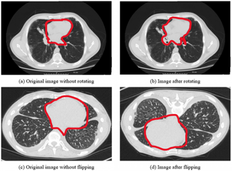
Figure 4. Showing the data augmentation on LuNa-16 dataset images before and after segmentation
Although the orientation of the microscope images does not vary, the sharpness of the target cell varies depending on where the microscope's focus plane is located. As consequence, by rotating, inverting, and filtering the image, we were able to extract additional information from it.
This was done in order to ensure that the number of better images for each of the three illness groups was equal for all three disease groups. As a consequence, there were twice as many images included in the final version as there were in the initial version. With a Gaussian filter with a standard deviation of three pixels, the images were enhanced, as was the edges with a convolutional edge enhancement filter that had a central weight of 5.4 and an 8-surrounding weight of 55% and improved the edges' appearance was shown in the Figure 4.
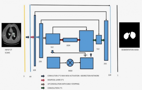
3.4 Network model architecture
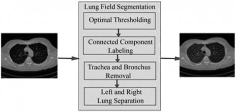
Pre-processing: The automatic lung segmentation approach is seen in Figure 5. In this stage, four critical processes are carried out: trachea and bronchus removal; optimum thresholding; connected component labelling; as well as separation of the left and right lungs. The procedure is detailed in the next section.
Figure 5. The block diagram of the proposed model
The lung parenchyma, trachea, and bronchial tree are all visible on the first CT scan of the lung. Fat, muscle, and bones may be seen on the exterior of the lung's anatomy. There are also nodules on the exterior of the lungs, which are called pulmonary nodules. In order to remove non-parenchymal tissues from a CT image, lung field segmentation must be performed. It is divided into many phases, which are as follows: The trachea and bronchi are removed by the use of a method known as region-growing. This is accomplished when the lung parenchyma has been separated from the surrounding architecture. After the left and right lungs have been put together, there are still certain pieces that need to be removed from the body.
Figure 6. The flow of the proposed architecture on the LuNa-16 dataset
When separating low density regions such as the lungs and airways from high density areas such as the chest, bones, fat, muscles, and pulmonary nodules (which have a high density of their own), the term "optimal thresholding" is used (non-body voxels). This technique is referred to as "optimal thresholding" (body-voxels). As seen in Figure 6, lung CT imaging reveals zones of low and high density. Instead of using a fixed threshold value, we employed optimal thresholding, which automatically determines the appropriate threshold for segmenting the data. This method significantly simplifies the task of accounting for minor variations in tissue density that may exist across different individuals. In order to determine the appropriate threshold, iterative approaches are used. To get things going, we employed repeated thresholding. If it was assumed that they were unsure of where to position the body voxels, this would be incorrect. There are no voxels that are not part of the body in this image. All of the other voxels in the image are part of the body. When the final run is completed, it displays the precise position of body and non-body voxels. Suppose that the threshold value is T at step t, which is what we'll state in the next paragraph. Initially, this threshold was utilised to distinguish between non-body and body voxels in the scene was shown in the Figure 7.
Figure 7. The proposed architecture for segmentation of bio-medical images
3.5 Loss function of proposed network model
The loss function is as follows:
$C(w, b)=\frac{1}{2 n} \sum_x\|y(x)-\|^2+\frac{1}{2 n} \lambda \sum_w W^2$ (25)
where, C, w, b, n, x, and an are the cost functions. It is used to do the back propagation process, which lowers the discrepancy between anticipated and actual values, hence increasing the accuracy of the process. The DNN is used to perform the back propagation [25] process. It is critical not to overtrain during the training phase, which is why the last item of the loss function divides the sum of all weights by 2n, which is equal to 2. Another method of preventing overfitting is to drop out. Some neurons are randomly hidden before back propagation, and the parameters are not changed as a result of the masked neurons. In order for the DNN to handle a large amount of data, it also requires a large amount of memory. This is due to the fact that the DNN requires a large amount of data. As a result, when a min batch is executed, a back propagation is carried out in order to allow for more rapid parameter changes. The activation function of the neural network is known as Leaky ReLU, and it is responsible for helping it simulate objects that are not straight lines. The activation function of the ReLU is represented by the following mathematical formula.
$y=\left\{\frac{x}{o} i f x>0 ; x<0\right.$ (26)
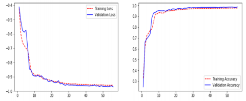
Figure 8. The loss function of the proposed classifier
In the example below, x represents the outcome of priority-weighted multiplication and paranoid addition, while y represents the output of an activation function, as indicated in the Figure 8. If x is less than zero, the answer is zero; if x is more than zero, the answer is one. Therefore, ReLU is capable of resolving the issue of the sigmoid activation function's gradient [26]. Weights cannot be modified indefinitely, however, since training is always being updated, which is referred to as "neuronal death" in the scientific community. The output of ReLU, on the other hand, is larger than zero, indicating that the output of the neural network has been modified. The usage of leaky ReLUs might be utilised to overcome the concerns described above. The activation function for the Leaky ReLU is represented by the following formula.
3.6 Activation function
An activation function is used by a Neural Network to take use of the concept of non-linearity. In order for the network to be properly trained and evaluated, this function must be used. Over the years, a large number of activation functions have been developed, but only a small number of them are actually employed in the majority of situations. ReLU, TanH (Tan Hyperbolic), Sigmoid, Leaky ReLU, and Swish are examples of such algorithms [27].
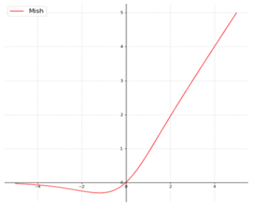
This work introduces a novel activation function, denoted by the letters Mish. Mish may be calculated using the formula f(x)=softplus(x) tanh. In a wide range of various kinds of deep networks and difficult datasets, the researchers discovered that Mish beats both ReLU and Swish, as well as other well-known activation functions, according to the findings.
Squeeze Excite Net-18's network with Mish performed better than the network with Swish and ReLU when it came to the classification test for the CIFAR 100 classification. Because Mish and Swish are so similar, it is simple for researchers and developers to include Mish into their Neural Network Models. Mish also performs better and is simpler to set together than other options.
Figure 9. Mish activation performance with respective to the ReLu
Mish's characteristics, such as being unbounded above and below, smooth, and nonmonotonic, all contribute to his superior performance when compared to other activation functions. As a result of the wide variety of training conditions available, it is difficult to determine why one activation function performs better than another, Figure 9 depicts a large number of activation functions. The graphs of Mish activation are shown next to them.
Figure 10. The performance of the MISH activation with respective to other activation functions
For example, as seen in Figure 10, owing of Mish's non-monotonic property, tiny negative inputs are maintained as negative outputs, which improves the expression and gradient flow. Due to the fact that the order of continuity of Mish is infinite, it has a significant advantage over ReLU, which has an order of continuity of 0. Due to this, ReLU cannot be continuously differentiable, which may make gradient-based optimization more challenging for those that employ it.
Figure 11. The sharp transition between the ReLU and MISH
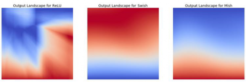
Due to the fact that Mish is a smooth function, it is easy to optimise and generalise, which is why the results became better with time. To determine how well ReLU, Swish, and Mish performed, the output landscape of a five-layer, randomly-initialized neural network was examined for each of them. In Figure 11, you can see how rapidly the scalar magnitudes for ReLU coordinates shift from Swish and Mish to the current figure. Because of this, a network that is simpler to regulate has smoother transitions, which in turn results in loss functions that are smoother. This makes it simpler to generalise the network, which is why Mish performs better than ReLU in several domains compared to ReLU. The landscapes of Mish and Swish, on the other hand, are very similar in this regard.
Additionally, complementary labelling is used in U-Net training. Two-dimensional data should be treated similarly to one-dimensional data. The model seeks to eliminate as many labelling mistakes as feasible in both directions. By comparison, the mass of each pixel decreases with time. Engaging with them accomplishes the two-fold objective.
In Table 2, we compare the results of numerous approaches on our test data with and without pre-processing (with CLAHE, wiener filter, and ROI segmentation). The table's sensitivity improves from 90% to 91% after pre-processing, and the dice coefficient increases from 91% to 92%.
This study examines a variety of labeling strategies, both monolithic and hybrid. The term "mono" refers to a single label input, while "hybrid" refers to a single label input with either a positive or negative output (complementary labeling) (complementary labeling). Regardless matter whether the model is trained on positive or negative ground truth, the output can never be better than the mono input. Complementary labeling seems to be ineffective when dealing with large data sets.
This research examines data from a variety of sources and includes 472 and 50 occurrences, respectively. Complementary labeling and pre-processing, as demonstrated in Table 3, outperform mono input in the majority of cases. On the other hand, complementary labeling is ineffective in the absence of pre-processing.
When dealing with little amounts of data, complementary labeling may be quite beneficial. As a result, this research examines the viability of labeling enhancement. Hybrid negatives are preferred over mono-input positives because smaller data volumes are more sensitive to hybrid negatives. Positive mono outputs provide a value of 90%, whereas negative hybrid inputs produce a value of 92% and the output of the results can be seen in Figure 12. If the data set is insufficient, more labels may be necessary to round.
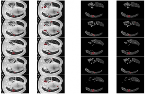
Figure 12. The ground truth prediction before segmentation and after segmentation
Table 2. The evaluation report of the different lung nodule semantic segmentation with comparison to our proposed algorithm
|
Evaluation |
Jiao et al. [7] |
Two-Parameter U-NET Model |
Three-Parameter U-NET Model |
|
Dice coefficient |
95.67% |
97.3% |
|
|
Confusion matrix |
Accuracy:95.67% |
Accuracy: |
Accuracy:97.3% |
|
Sensitivity:93.45% |
Sensitivity: |
Sensitivity:96.5% |
|
|
Specificity:92.15% |
Specificity: |
Specificity:94.1% |
Table 3. Valuation of the different semantic lung nodule segmentation with comparison to our proposed algorithm
|
Valuation |
Three-Parameter U-NET Model |
Two-Parameter U-NET Model |
|
Dice coefficient |
97.3% |
|
|
Confusion matrix |
Accuracy:97.3% |
Accuracy: |
|
Sensitivity:96.5% |
Sensitivity: |
|
|
Specificity:94.1% |
Specificity: |
Table 4. The evaluation of the lung nodule semantic segmentation on a small% age of the LUNA-16 images
|
Evaluation |
Eali et al. [10] |
Two-Parameter U-NET Model |
Three-Parameter U-NET Model |
|
Dice coefficient |
96.15% |
97.3% |
|
|
Confusion matrix |
Accuracy: 95.15% |
Accuracy: |
Accuracy:97.3% |
|
Sensitivity: 96.23% |
Sensitivity: |
Sensitivity:96.5% |
|
|
Specificity: 95.15% |
Specificity: |
Specificity:94.1% |
The U-NET algorithm for the lung tumor segmentation model has been implemented in TensorFlow and tested its efficiency for image segmentation. The LUNA-16 images are considered for image segmentation. The performance of both two-parameter and three-parameter logistic type distributions was shown in the Table 4 and Table 5 respectively.
Table 5. The valuation of the lung nodule semantic segmentation on a small% age of the LUNA-16 images
|
Evaluation |
Rao et al. [24] |
Two-Parameter U-NET Model |
Three-Parameter U-NET Model |
|
Dice Coefficient |
96.15% |
97.3% |
|
|
Confusion matrix |
Accuracy: 95.15% |
Accuracy: |
Accuracy:97.3% |
|
Sensitivity: 96.23% |
Sensitivity: |
Sensitivity:96.5% |
|
|
Specificity: 95.15% |
Specificity: |
Specificity:94.1% |
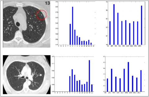
Figure 13. Example of the pixel intensities of the lung nodule CT scan images of benign and malignant nodules
The histograms of the pixel intensities of the CT scan images are shown in Figure 13.
From the Table 6, it was very clear that our classifier SENETS-Grad-Cam++ has outperformed remaining all the classifiers in terms of the performance metrics like AUC and accuracy on LUNA 16 benchmark dataset.
From the Table 7, it was clearly evident that our method was performed very well with few samples size from LUNA 16 dataset. The results clearly shows that out proposed model and method are good at classifying odd benign and Malignant tumours was shown in the Figure 14. As, a result the model has achieved a trust gain when compared with various others methods.
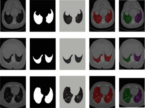
Figure 14. The proposed classifier on LuNa-16 dataset. Second column showing the original image, third column showing the lung lode, and last two is the segmented image
Table 6. Evaluation of proposed with other procedures based on handcrafted structures
|
Author’s |
Year |
Features |
Classifier |
Database |
Samples |
AUC |
Accuracy |
|
Gao et al. [5] |
2022 |
Intrinsic |
3D-CNN |
LIDC |
87 |
95.57% |
95.53% |
|
Joshua et al. [6] |
2022 |
Wrapper |
CNN |
LIDC |
1407 |
- |
92.20% |
|
Jiao et al. [7] |
2022 |
Filter Methods |
ResNet-19 |
LIDC |
1407 |
- |
90.68% |
|
Krishnamacharya et al. [8] |
2022 |
Intrinsic |
LSTM |
LIDC |
1179 |
86.69% |
79.35% |
|
Li et al. [9] |
2022 |
Wrapper |
DCNN |
LIDC |
160 |
- |
94.89% |
|
Lieanto et al. [11] |
2023 |
Intrinsic |
CNN |
LIDC |
1366 |
92.34% |
91.13% |
|
Liu et al. [12] |
2022 |
Filter Methods |
ResNet-16 |
LIDC |
572 |
65.56% |
91.13% |
|
Qiu et al. [14] |
2022 |
Intrinsic |
MD-CNN |
LIDC/LUNA16 |
1201 |
96.64% |
97.08% |
|
Proposed Model U-NET with Three Parameters Logistic |
LIDC/LUNA16 |
1506 |
96.89% |
97.89% |
|||
Table 7. Assessment of the proposed methods with other approaches based on deep learning topographies
|
Authors |
Year |
Method |
Database |
Samples |
AUC |
Accuracy |
|
Rao et al. [15] |
2022 |
Convolutional Neural Network |
LIDC |
2619 |
91.45% |
90.15% |
|
Seitz et al. [16] |
2022 |
Deep CNN with Autoencoders |
LIDC |
487 |
77.89% |
- |
|
Son et al. [17] |
2022 |
CNN with Gradient Descent |
LIDC |
890 |
96.58% |
90.91% |
|
Joshua et al. [18] |
2022 |
Generative Adversarial Networks+CNN |
LIDC |
2889 |
95.67% |
93.85% |
|
Tang et al. [19] |
2022 |
CNN with Self Organizing Maps |
LIDC |
1200 |
- |
91.44% |
|
Rao et al. [24] |
2022 |
Recurrent Neural Networks |
LIDC |
60 |
94.40% |
90.58% |
|
Bhattacharyya et al. [27] |
2022 |
RNN + GANs |
LUNA16 |
1230 |
96.64% |
97.08% |
|
Proposed Model U-NET with Three Parameters Logistic |
LuNa-16 |
1506 |
96.89% |
97.89% |
||
For the purposes of this research, we used improvised U-NET and limited EM with Logistic type distribution for the (U-NET+three parameter logistic distribution) to make it simple to distinguish between various portions of the lung field. It makes use of the spatial interaction of neighbouring voxels to create images that are visually distinct. This approach was used to mimic the U-NET+Three parameter logistic distribution algorith, the hierarchal clustering algorithm is used to obtain the number of components in the mixture model and initializem, which has two parameters. Two parameter type distribution is utilised to segregate lung and chest voxels from one another in the H matrix using the U-NET+Three parameter logistic distribution technique and the U-NET+Three parameter logistic distribution method. When we compared our approach to four other lung segmentation methods, we discovered that ours was the most successful. We employed 40 patients from two separate datasets to evaluate this. In terms of DSC performance, the findings demonstrate that the suggested technique outperforms the other strategies by a significant margin. Current evidence suggests that the approach recommended works effectively for simple to medium-sized situations Our procedure, on the other hand, may not be effective if the lungs are really ill. Our next research project will look at how to create algorithms that can distinguish between extremely good and very awful CT scans images.
The assessment performed in this research enables for further development of the concepts identified in this study, which may be used to the construction of a high-accuracy CAD system. Based on this research, it is possible that future research will go the following routes.
·In order to increase the accuracy and robustness of this tool's classification of all other forms of lung nodules in the future, we will seek to improve its accuracy and robustness for all other types of nodules.
·To determine if the suggested approach can be utilised as a therapy, it will be evaluated on a variety of datasets in the near future.
·In the future, it will be able to classify nodules according to their characteristics. This will be included into the framework for segmenting lung nodules.
·To devise a method of dividing lung nodules of varying shapes and sizes into smaller pieces. Research and development of an automated technology to assist radiologists in the detection and screening for lung cancer.
·Interstitial lung disease, pleural effusions, and consolidations are all examples of lung illnesses that might occur in the future. The data could be used to forecast when these diseases would occur.
This research was financially supported by the Ministry of Small and Medium-sized Enterprises (SMEs) and Startups (MSS), Korea, under the “Regional Specialized Industry Development Plus Program (R&D, S3246057)” supervised by the Korea Technology and Information Promotion Agency for SMEs (TIPA).
[1] Bhakkan-Mambir, B., Deloumeaux, J., Luce, D. (2022). Geographical variations of cancer incidence in Guadeloupe, French West Indies. BMC cancer, 22(1): 1-9. https://doi.org/10.1186/s12885-022-09886-6
[2] Eali, J., Neal, S., Bhattacharyya, D., Nakka, T.R., Hong, S.P. (2022). A novel approach in bio-medical image segmentation for analyzing brain cancer images with U-NET semantic segmentation and TPLD models using SVM. Traitement Du Signal, 39(2): 419-430. https://doi.org/10.18280/ts.390203
[3] Chang, J., Han, K.T., Medina, M., Kim, S.J. (2022). Palliative care and healthcare utilization among deceased metastatic lung cancer patients in US hospitals. BMC Palliative Care, 21(1): 1-8. https://doi.org/10.1186/s12904-022-01026-y
[4] Fujiwara, T., Nakata, E., Kunisada, T., Ozaki, T., Kawai, A. (2022). Alveolar soft part sarcoma: progress toward improvement in survival? A population-based study. BMC Cancer, 22(1): 891. https://doi.org/10.1186/s12885-022-09968-5
[5] Gao, C., Kong, N., Zhang, F., Zhou, L., Xu, M., Wu, L. (2022). Development and validation of the potential biomarkers based on m6A-related lncRNAs for the predictions of overall survival in the lung adenocarcinoma and differential analysis with cuproptosis. BMC Bioinformatics, 23(1): 1-18. https://doi.org/10.1186/s12859-022-04869-7
[6] Joshua, E.S.N., Bhattacharyya, D., Rao, N.T. (2022). The use of digital technologies in the response to SARS-2 CoV2-19 in the public health sector. Digital Innovation for Healthcare in COVID-19 Pandemic, 391-418. https://doi.org/10.1016/B978-0-12-821318-6.00003-7
[7] Jiao, Z., Feng, X., Cui, Y., Wang, L., Gan, J., Zhao, Y., Meng, Q. (2022). Expression characteristic, immune signature, and prognosis value of EFNA family identified by multi-omics integrative analysis in pan-cancer. BMC Cancer, 22(1): 871. https://doi.org/10.1186/s12885-022-09951-0
[8] Krishnamachari, K., Lu, D., Swift-Scott, A., Yeraliyev, A., Lee, K., Huang, W., Leng, S.N., Skanderup, A.J. (2022). Accurate somatic variant detection using weakly supervised deep learning. Nature Communications, 13(1): 4248. https://doi.org/10.1038/s41467-022-31765-8
[9] Li, Q., Wang, R., Yang, Z., Li, W., Yang, J., Wang, Z., Bai, H., Cui, Y.L., Tian, Y.H., Wu, Z.X., Guo, Y.Q., Xu, J.C., Wen, L., He, J., Tang, F., Wang, J. (2022). Molecular profiling of human non-small cell lung cancer by single-cell RNA-seq. Genome Medicine, 14(1): 1-18. https://doi.org/10.1186/s13073-022-01089-9
[10] Eali, S.N.J., Rao, N.T., Swathi, K., Satyanarayana, K.V., Bhattacharyya, D., Kim, T. (2018). Simulated studies on the performance of intelligent transportation system using vehicular networks. International Journal of Grid and Distributed Computing, 11(4): 27-36. https://doi.org/10.14257/ijgdc.2018.11.4.03
[11] Lieanto, C., Putra, I.M.R., Lathifa, U.S., Arief, M.O.V., Fuad, M., Hertiani, T. (2023). Bioinformatics study: Syzygium samarangense leaves chalcone extract as lung cancer proliferation inhibitor. Biointerface Research in Applied Chemistry, 13(2): 173. https://doi.org/10.33263/BRIAC132.173
[12] Liu, L., Gu, M., Ma, J., Wang, Y., Li, M., Wang, H., Yin, X., Li, X. (2022). CircGPR137B/miR-4739/FTO feedback loop suppresses tumorigenesis and metastasis of hepatocellular carcinoma. Molecular Cancer, 21(1): 149. https://doi.org/10.1186/s12943-022-01619-4
[13] Luo, D., Feng, W., Ma, Y., Jiang, Z. (2022). Identification and validation of a novel prognostic model of inflammation-related gene signature of lung adenocarcinoma. Scientific Reports, 12(1): 14729. https://doi.org/10.1038/s41598-022-19105-8
[14] Qiu, X., Liu, W., Zheng, Y., Zeng, K., Wang, H., Sun, H., Dai, J. (2022). Identification of HMGB2 associated with proliferation, invasion and prognosis in lung adenocarcinoma via weighted gene co-expression network analysis. BMC Pulmonary Medicine, 22(1): 1-16. https://doi.org/10.1186/s12890-022-02110-y
[15] Rao, C.V., Xu, C., Zhang, Y., Asch, A.S., Yamada, H.Y. (2022). Genomic instability genes in lung and colon adenocarcinoma indicate organ specificity of transcriptomic impact on Copy Number Alterations. Scientific Reports, 12(1): 11739. https://doi.org/10.1038/s41598-022-15692-8
[16] Seitz, R.S., Hurwitz, M.E., Nielsen, T.J., Bailey, D.B., Varga, M.G., Ring, B.Z., Metts, C.F., Schweitzer, B.L., McGregor, K., Ross, D.T. (2022). Translation of the 27-gene immuno-oncology test (IO score) to predict outcomes in immune checkpoint inhibitor treated metastatic urothelial cancer patients. Journal of Translational Medicine, 20(1): 1-11. https://doi.org/10.1186/s12967-022-03563-9
[17] Son, S.U., Kim, H.W., Shin, K.S. (2022). Structural identification of active moiety in anti-tumor metastatic polysaccharide purified from fermented barley by sequential enzymatic hydrolysis. Food Bioscience, 50: 101999. https://doi.org/10.1016/j.fbio.2022.101999
[18] Joshua, E.S.N., Bhattacharyya, D., Chakkravarthy, M. (2021). Lung nodule semantic segmentation with bi-direction features using U-INET. Journal of Medical pharmaceutical and allied sciences, 10(5): 3494-3499. https://doi.org/10.22270/jmpas.V10I5.1454
[19] Tang, Y.L., Li, G.S., Li, D.M., et al. (2022). The clinical significance of integrin subunit alpha V in cancers: from small cell lung carcinoma to pan-cancer. BMC Pulmonary Medicine, 22(1): 300. https://doi.org/10.1186/s12890-022-02095-8
[20] Trembecki, Ł., Sztuder, A., Dębicka, I., Matkowski, R., Maciejczyk, A. (2022). The pilot project of the national cancer network in Poland: Assessment of the functioning of the National Cancer Network and results from quality indicators for lung cancer (2019–2021). BMC Cancer, 22(1): 1-10. https://doi.org/10.1186/s12885-022-10020-9
[21] Turner, E., Johnson, E., Levin, K., Gingles, S., Mackay, E., Roux, C., Milligan, M., Mackie, M., Farrell, K., Murray, K., Adams, S., Brand, J., Anderson, D., Bayes, H. (2022). Multi-disciplinary community respiratory team management of patients with chronic respiratory illness during the COVID-19 pandemic. NPJ Primary Care Respiratory Medicine, 32(1): 26. https://doi.org/10.1038/s41533-022-00290-y
[22] Yang, M., Lin, C., Wang, Y., Chen, K., Zhang, H., Li, W. (2022). Identification of a cytokine-dominated immunosuppressive class in squamous cell lung carcinoma with implications for immunotherapy resistance. Genome Medicine, 14(1): 72. https://doi.org/10.1186/s13073-022-01079-x
[23] Zhang, H., Udugamasooriya, D.G. (2022). Optimization of a cell surface vimentin binding peptoid to extract antagonist effect on lung cancer cells. Bioorganic Chemistry, 129: 106113. https://doi.org/10.1016/j.bioorg.2022.106113
[24] Rao, N.T., Bhattacharyya, D., Joshua, E.S.N. (2022). An extensive discussion on utilization of data security and big data models for resolving healthcare problems. In Multi-Chaos, Fractal and Multi-fractional Artificial Intelligence of Different Complex Systems, pp. 311-324. https://doi.org/10.1016/B978-0-323-90032-4.00001-8
[25] Zhang, Y., He, X., Gao, H. (2022). KMT2C mutation in a Chinese man with primary multidrug-resistant metastatic adenocarcinoma of rete testis: A case report. BMC Urology, 22(1): 1-6. https://doi.org/10.1186/s12894-022-01075-8
[26] Doppala, B.P., NagaMallik Raj, S., Stephen Neal Joshua, E., Thirupathi Rao, N. (2021). Automatic determination of harassment in social network using machine learning. In Smart Technologies in Data Science and Communication: Proceedings of SMART-DSC 2021, pp. 245-253. https://doi.org/10.1007/978-981-16-1773-7_20
[27] Joshua, E.S.N., Bhattacharyya, D., Rao, N.T. (2022). Managing information security risk and Internet of Things (IoT) impact on challenges of medicinal problems with complex settings: a complete systematic approach. In Multi-Chaos, Fractal and Multi-fractional Artificial Intelligence of Different Complex Systems, pp. 291-310. https://doi.org/10.1016/B978-0-323-90032-4.00007-9