Furkan Balcı![]()
© 2024 The author. This article is published by IIETA and is licensed under the CC BY 4.0 license (http://creativecommons.org/licenses/by/4.0/).
OPEN ACCESS
For detecting and classifying brain tumors, clinicians use Magnetic Resonance Imaging (MRI) data. Automated AI-powered tools accelerate the diagnostic process for clinicians. However, large amounts of data are needed for these models to achieve high accuracy. Variational Autoencoders (VAE) and Generative Adversarial Networks (GAN) architecture are combined for dataset expansion. The accuracy was improved with the artificial image set created in all tested models. However, since the accuracy rate remained at 92,960% using Long Short Term Memory Algorithm, it was observed that a hybrid method was also needed, and hybrid Elmann Bidirectional Long Short Memory Algorithm (Elmann-BiLSTM) was developed. In this proposed approach based on deep learning, a Guided Bilateral Filter is used to separate skull from images after VAE-GAN structure. The thresholding scheme extracts tumour regions from the original image in parts. Edge features and major texture data are collected from these tumor images produced using the Improved Gabor Wavelet Transform. Random Forest-based feature selection algorithm will select optimal features that increase accuracy from extracted features. These features feed the Elmann-BiLSTM algorithm used as a two-step classifier. The accuracy rate was 98.897% in the one-step classification approach and 100% and 99.313% in the two-step classifier approach, respectively.
variational auto-encoder, Generative Adversarial Networks (GAN), brain tumor classification, deep learning, Elmann RNN
Developments in diagnosis, with the spread of artificial intelligence, provide various conveniences for clinicians in examining long data. Especially for image data, automatic approaches are being developed for clinicians to determine the type of disease and to identify diseased areas. One of the most aggressive of these diseases is cancer [1]. Brain cancer is uncontrolled and irregular protein growth in or around the brain tissue. This growth pressures other brain parts, preventing the brain from performing its normal functions. These tumors formed in the brain are grouped under two headings: benign tumors and malignant tumors. Benign brain tumors are divided into different categories and named. Some of these can be listed as pituitary adenoma, neurofibroma, craniopharyngioma, schwannoma, dysembryoplastic neuroepithelial tumor, choroid plexus tumor, glioma, glioblastoma, nasopharyngeal angiofibroma. Types of malignant tumors are the most aggressive. In the literature, these malignant tumors are called brain cancer in Layman's terms. If the uncontrolled growth of protein tissue breaks the coating and covers to other part of body or tissue, it is named cancer [2]. Cancers can spread to different regions due to metastasis [3]. If a tumor occurs directly in the brain, it is called a primary brain tumor. If it happens in different parts of the body or tissue, such as liver or lung tumors and then occurs in the brain lobes, it is called brain metastasis [4]. Some clinicians refer to brain metastasis as secondary brain tumor [4]. The brain's tumours are classified into three classes, namely “pituitary, meningioma and glioma”, according to their formation sites. The pituitary is an endocrine gland weighing about 0.5 grams located in the lower layer of the brain [5]. Any abnormal protein growth around the pituitary is called a pituitary brain tumor. Meningioma develops more slowly than other tumors and is a benign tumor. Meningioma is usually located in the brain's outer covering under the skull. Glioma is a tumour that is more aggressive and malignant than the other two types. This species causes a higher mortality rate [6]. Gliomas can occur at different points regionally. Glioma tumors are usually a more difficult type of tumor to diagnose than other types. The main reason for this is that these tumors occur in the cerebral hemispheres and the supporting tissues of the brain [5]. It is easier to detect tumor types by looking at the regions where they are seen in pituitary and meningioma tumors than in gliomas.
The World Health Organization (WHO) has separated brain tumors into three classes according to their origin in brain’s parts [7]. There are several tests (biomarkers, biopsies, imaging, and neurological examination) clinicians use for grade estimation and tumor diagnosis [8]. The chance of an early diagnosis of brain tumors is quite complex compared to other diseases. In the initial stages, symptoms such as headache and vomiting usually occur, but these symptoms are common symptoms of many diseases. Early diagnosis is often not possible because Positron Emission Tomography (PET), Computed Axial Tomography (CT) or Magnetic Resonance Imaging (MRI) is not requested from individuals with these symptoms [9]. Besides these symptoms, the most prominent symptom is increased intracranial pressure [9]. Since abnormal protein growth cannot naturally change the skull volume, intracranial pressure will increase. Generally, meningiomas, pituitary and benign tumors develop more slowly than malignant tumors. Because of their slow development, typical symptoms are not seen. Different psychological effects were seen in individuals with meningioma tumor. The most important examples of these psychological states are psychosis, memory loss, and sudden personality changes [10]. Psychological symptoms delay the diagnosis of diseases such as tumors. Generally, psychological symptoms are more common in meningiomas and benign tumors [11]. Symptoms vary in gliomas. Typically, patients present with seizures, fatigue, regional edema, and psychiatric disorders [12]. Therefore, some researchers emphasize that neuroimaging techniques should be used when psychiatric symptoms are encountered [10]. There are situations where each imaging technique is superior to the other. MR images have lower spatial resolution and longer imaging time than CT images [13]. Chest and bone scans require high spatial resolution. Therefore, CT is generally used in this imaging. However, MRI is used instead of CT because higher contrast is required for imaging performed in soft tissues [13]. Simple MRI fails to differentiate between benign and malignant tumors. Therefore, MRI with contrast is primarily preferred [14]. In order to avoid these problems, Perfusion-Weighted Imaging (PWI) method, which can produce perfusion maps, or Magnetic Resonance Spectroscopic Imaging (MRSI) techniques, which have significant contributions in detecting benign or malignant tumor tissue, are used [14].
Contrast-enhanced MRI is an important method for clinicians to monitor the tumor process of people with tumors. It is also used by clinicians and surgeons in surgical intervention planning. Contrast enhancement plays a crucial part in imaging. If contrast enhancement does not occur on early postoperative MRI, it is understood that the resection is complete [15]. Isocitrate dehydrogenase (IDH) is the enzyme involved in the tricarboxylic acid cycle. Tumors with normal IDH genes are termed as IDH negative [16]. However, with contrast-enhanced MRI, clinicians can make mistakes in evaluating patients with IDH-negative anaplastic glioma [17]. IDH-negative tumors are both the most aggressive type and do not change the contrast on MRI [15]. For this reason, positron emission tomography (PET) scans have been developed to fill this gap. Radioactive tracers are used in PET scans to monitor processes. Both metabolic and molecular processes can be followed in PET scans. 2-18F-fluorodeoxyglucose (18F-FDG) is the most widely used of the radioactive tracers. 18F-FDG is often used in oncology to diagnose peripheral tumors [14]. However, the proliferation marker 18F-3'-deoxy-3'-fluorothymidine (18F-FLT), which accumulates in cerebral gliomas in direct proportion to the degree of malignancy, is used in screening [18]. These tracers have some problems, such as the inability to cross the blood-brain barrier and high glucose metabolism levels in the brain. Therefore, PET scanning with radiolabeled amino acids is used as an alternative to contrast-enhanced MRI scanning [19]. O-(2-[18F] fuoroethyl)-L-tyrosine (FET) is the most commonly used radiolabeled amino acid in PET scans with radiolabeled amino acids, especially in Europe [20].
Although technological medical breakthroughs have significant results, the mortality rates in individuals with brain tumors are still relatively high [21]. These imaging techniques, which have developed with technological developments, help clinicians in diagnosis and classification. Artificial intelligence-based support systems are being developed to prevent possible clinician decision errors [22]. Thanks to computer-aided diagnostic systems, systems are being developed to assist neurologists and medical professionals. Automated artificial intelligence-based intelligent systems using biomedical data are prevalent today. The classification and diagnosis of brain tumors is also the research subject of artificial intelligence-based systems. Classification of brain tumor applications is one of the critical areas of medical research involving various complexities. Different machine learning classifiers are used for brain tumor detection [23]. Traditional machine learning algorithms and methods in the process of diagnosing and classifying brain tumors consists several process steps, including intensive pre-processing, feature extraction from MR images, and feature selection to select important features. Feature extraction and selection is one of the most critical steps affecting classification accuracy [24]. With the development and widespread use of deep learning-based algorithms and methods, the problem of manual feature selection in machine learning methods is eliminated, and high performance is shown in image-based studies [25-28]. In addition, deep learning algorithms and methods need dense and increased data to train hundreds of layers and millions of parameters. Different deep learning architectures (Stacked Autoencoders, Convolutional Neural Networks (CNN), Recurrent Neural Networks (RNN), Deep Boltzmann Machine (DBM), Long Short-Term Memory Networks (LSTM), Deep Belief Networks (DBN)) are used for image classification applications [29]. Some advanced deep learning models for image classification, such as DenseNet, and AlexNet, cause long processing times in computational complexity due to their extensive layers. Synthesized MRI/CT data are challenging and costly [30]. This problem can be solved with another deep learning method called Generative Adversarial Network (GAN). Developed by Goodfellow et al. in 2014, this method consists of a generator and discriminator [31]. These two components work in conjunction with each other. The generator or the generator part, in other words, uses the data it receives for training to produce fake data close to reality. On the other hand, the discriminative part categorizes the images produced by the generator as real or fake. While the image pixel is used to create pixels in the generators used before the GAN architecture, it performs learning on a whole image as input in the GAN architecture. GAN architecture is widely used in medical images. GAN architecture has been used for brain tumor segmentation [32, 33]. It is also used to obtain super-resolution magnetic resonance images [34].
Basic studies with machine learning and deep learning methods for brain tumor classification are frequently encountered in the literature. GAN architecture is commonly used primarily for the reproduction of image data. Different studies were developed using GAN due to the cost and difficulty of accessing medical data. However, the biggest problem encountered in these studies is mode collapse due to the small dataset. However, basic machine learning algorithms are discovered in the first literature studies. The number of studies in which deep learning-based or hybrid methods are used in automatic tumor classifier studies developed with inspiration from these studies is relatively high. In classical studies, the segmentation process can usually be used. Although this process improves accuracy, it has pretty time-consuming processing times [35]. Therefore, processing time can be considered as limiting for the designed studies. In brain tumor classification, complex architectures must be combined and operated in harmony. CNN, one of the deep learning architectures, is generally used for classification in the literature. The idea of producing synthetic data is widely used, primarily due to the problems experienced in collecting medical data. Liu et al. proved that the GAN architecture can be used for data augmentation by testing using CT images [36].
There are many datasets in the literature apart from the datasets used in this study. Nguyen et al. propose a combined DCCN-BiFPN model to increase classification accuracy using the dataset called classification BraTS 2020 [37]. In this way, it is argued that the accuracy performance is improved. In addition, in some studies, different datasets are combined and used to classify tumour type and stage. Ayadi et al. use the CNN architecture, combining the Figshare and Radiopaedia datasets, to classify tumour type and stage [38]. Zhou et al. [39] used CNN architecture using data obtained from different axial sections while classifying tumors. In similar studies, the performance is generally increased by combining or hybridizing the models. However, classical methods such as Random Forest, CNN, and Fourier Convolutional Neural Network (FCNN) were also used in most studies. In a study using these algorithms, Paul et al. [40] achieved the highest accuracy of 90.26% with the CNN architecture. Abiwinanda et al. [41] tested the parameters of the CNN architecture with seven different models and reached an accuracy of 84.19%. Ge et al. [42] used the CNN architecture to determine the tumor grade of glioma. Rahman and colleagues [43] performed tumor classification with MRI images using three different CNN-based (VGGNet, AlexNet, GoogleNet) architectures with overfitting reduction.
One of the most critical operations of classification studies on image data is pre-processing techniques. In some studies in the literature, various pre-processing methods are used to improve classification results. For example, Tahir et al., using noise reduction, contrast enhancement and edge detection methods from these improvement studies, increased the classification accuracy to 86% with SVM architecture on the Figshare dataset [35].
In addition, the statistical properties of image data are a vital issue for artificial intelligence-based studies. There are various feature extraction approaches from image data. However, transformations such as Wavelet transform can be used in both 2D and 3D images. In their study of Ismail, various statistical properties reached 91.9% accuracy by using 2D discrete wavelet transform and Gabor filter [44]. Ayadi et al. [38] extracted classical features and then applied a feature selection algorithm to select certain main features. When the studies in the literature are examined, this study is designed to eliminate the shortcomings of a fully comprehensive automatic classifier. In the proposed method, a small number of data taken as input is amplified. In addition, there is a feature extractor and feature selector architecture in its structure to determine the features and select the optimum features. Finally, thanks to the two-step hybrid classifier aim to increase the accuracy percentage in classifying healthy individuals.
GAN architecture can be used to solve the problem of high data need in deep learning algorithms. Classical generators generally generate new data by adding random Gaussian noise to the input data. Since random Gaussian noise has a lower disturbance than most noise types, the generator part produces blurred and similar image data. These blurry images created cannot reveal realistic features for deep learning architectures. Furthermore, the images produced by such generators may not help work on MR or PET images. To solve this problem, the dataset needs to be augmented. Synthetic MR and PET images are produced by proposing a combined method in this study to augment the dataset. In solving this, the Variational Automatic Encoder (VAE) and the Generative Adversarial Network (GAN) are combined. Hybrid models resulting from the combination of suitable models achieve higher accuracy rates. Therefore, a hybrid model was developed as a classifier as an important contribution in this study. In addition to these problems, a two-step classification system has been developed to solve the harmful effects of the increase in the number of classifications on success. In this developed system, first of all, the presence of the tumor is determined in the first hybrid classifier step. The test image will be transferred to the second classifier if the tumour is detected. The second hybrid classifier classifies the tumor type. The contributions of the proposed study to the literature are as follows:
The rest of this article: Information about the mathematical approach of the proposed two-step hybrid Elmann-BiLSTM classifier in the second part, and in the last two parts, the test results of the proposed two-step hybrid Elmann-BiLSTM classifier are examined and discussed, and information about the results are shared.
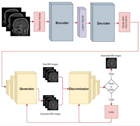
This section will explain the details of the proposed approach that makes hybrid deep learning-based brain tumor detection from MR images. The algorithm is terminated in this two-step classification approach if the first classifier does not detect a tumor. If the first classifier detects a tumor, the input data will be transferred to the second classifier, and the tumor type will be detected. The proposed approach combines two proven successful methods: the combined VAE-GAN data augmentation approach and the Hybrid Elmann-BiLSTM classifier. First, the cerebral lobes are separated from the skull. In the next part, a method combining VAE and GAN architectures is used to augment the dataset needed by the deep learning architecture. This way, the intensive data need for deep learning architecture is met. The VAE architecture is an encoder-decoder network architecture. In the proposed method, after the VAE architecture is trained, its structure is updated as a decoder-encoder, and non-random noise is added to the image (with image manifold information). Generally, sampling is performed using random Gaussian noise in GAN architecture. However, the GAN structure is sampled in this proposed architecture instead of using the noise vectors produced by the VAE architecture. This way, mode collapse, frequently encountered when using fewer data in GAN architecture, will be prevented. If this situation could not be prevented, the GAN architecture would no longer be able to produce different images. Images detected as real images in Discriminator output are used as a dataset. A Guided Bilateral Filter (GBF) filters the noises from the MRI images in the augmented dataset. Before performing the segmentation, a threshold level should be determined by considering the gray levels. Improved Gabor Wavelet Transform (IGWT) is used for feature extraction from edge of segments. In this way, meaningful features will be obtained from the extracted segments. Feature selection will be needed to increase the performance of the classification algorithm from the extracted features. The most convenient features will be optimized for feature selection using a binary Random Forest-based feature selector algorithm. All these processes basically constitute the preparatory steps for the classification algorithm. A hybrid algorithm was designed as the classification algorithm. In this algorithm, Elmann-RNN architecture and Bi-LSTM architecture are hybridized. In this study, the hybrid model will be named Elmann-BiLSTM. The classification process will be carried out in two steps. The first classifier will decide whether the tumor is present or absent. The second classifier algorithm is the classifier that selects which tumor is the result of the first classifier if there is a tumor. The flow chart of the proposed combined VAE-GAN and hybrid Elmann-BiLSTM architecture is shown in Figure 1.
Figure 1. Overall structural design of the proposed method
Figure 2. Sample MR images from the Dataset A and Dataset B. a: healthy, b: glioma, c: meningioma, d: pituitary
2.1 Dataset
In this study, training and testing steps were carried out using the combination of two different datasets to measure the accuracy of the designed architecture. These datasets will be referred to as “Dataset A” and “Dataset B”. First, the dataset called Dataset A is the dataset publicly shared by Cheng et al. [45]. This dataset contains 3064 MRI images from 233 subjects. In addition, there are data according to the types of glioma, meningioma, and pituitary, which are the subject of this study. Two-dimensional MR data of these three types of brain tumors were recorded in the axial, coronal and sagittal axes. However, there is no data from healthy subjects in this dataset. Therefore, a different dataset is needed for the disease-healthy classification. In addition, the dataset was augmented for all three tumor types. Dataset B is a publicly available dataset on the Kaggle site [46]. Unlike Dataset A, Dataset B also includes MR images of healthy individuals. This way, the proposed method's first classifier can classify the patient-healthy. This dataset contains 3264 images collected from subjects with tumors and healthy subjects. Figure 2 contains sample images of these datasets.
2.2 Combined variational autoencoders – Generative Adversarial Networks architecture
The variational autoencoder (VAEs) architecture is a deep learning architecture that reconstructs the data it takes as input and produces outputs with the backpropagation principle. Unlike standard autoencoder architectures, Variational autoencoder architecture uses a probability model in deep networks to provide balance types. The distribution of neurons in the hidden layers is forced to be distributed according to the normal distribution. Kullback-Leibler (KL) loss was used during VAE training to measure the difference between the distribution of latent variables and the target distribution (usually the normal distribution). KL loss indicates how close the resulting distribution of latent variables is to the target distribution. This loss function encourages latent variables to be distributed close to the normal distribution. Variational autoencoders have three basic components in their structure: encoder, decoder and loss function.
These structures allow variational autoencoder architecture to produce complex models using datasets. In the input layer, standard deviation and mean the encoder block creates vectors from the data ($\left\{ {{x}_{i}} \right\}_{i=1}^{N}$) sent as input to the structure. These vectors are created for use in hidden layers ($z$). The hidden layer generates a random new data ($\left\{ {{{\tilde{x}}}_{i}} \right\}_{i=1}^{N}$) similar to the input data ($\left\{ {{x}_{i}} \right\}_{i=1}^{N}$) in the input layer. Input $x$ and the $\tilde{x}$ data generated from this X input are larger in size than the hidden variable $z$. $\theta $ and $\varphi $ represent weights and biases values respectively. There is a distribution function for each feature in this hidden layer in the Variational autoencoders architecture. The data is produced by the directed model $P(x|z)$. The encoder learns the $q(x|z)$ approach and uses it in the ${{P}_{\theta }}(x|z)$ posterior distribution. Thanks to the objective function shown in Eq. (1), variational autoencoders architecture differs from other autoencoder architectures. The ${{\mathbb{E}}_{z \sim q(z|x)}}\left[ log{{P}_{\theta }}(x|z) \right]$ expression basically represents the probability of reconstructing from the input data. The ${{D}_{kl}}\left[ q(z|x){{P}_{\theta }}\left( z \right) \right]$ expression, on the other hand, aims to create a $q$ distribution similar to the previous $P$ distribution.
$\mathcal{L}=-{{\mathbb{E}}_{z \sim q(z|x)}}\left[ log{{P}_{\theta }}(x|z) \right]+{{D}_{kl}}\left[ q(z|x){{P}_{\theta }}\left( z \right) \right]$ (1)
${{F}_{1}}$ and ${{F}_{2}}$ represent the mapping function of the encoder and decoder blocks.
${{F}_{1}}:~{{x}_{i}}\to {{z}_{i}},~{{x}_{i}} \sim P\left( x \right),~{{z}_{i}} \sim N\left( 0,i \right),~i=1,2,3,\ldots ,~N$ (2)
${{F}_{2}}:~{{z}_{i}}\to {{x}_{i}},~{{x}_{i}} \sim P\left( x|z \right)$ (3)
Using Eq. (1):
${{F}_{1}},{{F}_{2}}=argmi{{n}_{{{F}_{1}},{{F}_{2}}}}\sum {{D}_{kl}}\left[ q\left( {{z}_{i}}\text{ }\!\!|\!\!\text{ }{{x}_{i}} \right)||{{P}_{\theta }}\left( {{z}_{i}} \right) \right]-{{\mathbb{E}}_{z \sim q(z|x)}}\left[ log{{P}_{\theta }}({{x}_{i}}|{{z}_{i}}) \right]$ (4)
If the encoder-decoder structure in this equation is converted to decoder-encoder:
${{F}_{1}}:~{{z}_{i}}\to {{x}_{i}},~{{z}_{i}} \sim N\left( 0,i \right),~{{x}_{i}} \sim P\left( x|z \right)$ (5)
${{F}_{2}}:~{{x}_{i}}\to {{z}_{i}},~{{z}_{i}} \sim N\left( 0,i \right)$ (6)
${{z}_{i}}$ in Eqs. (5) and (6) represents the noise distribution. The new noise vector will be sampled using informative noise as input in this reconstructed architecture. Thanks to this vector, new image data can be produced from the image used as input. However, this method falls short in augmentation medical imaging data. In this proposed approach, meaningful data reproduction is aimed by combining the GAN architecture, which is the most modern version of the productive architectures, and the VAE architecture. GAN architecture basically consists of two parts: generative block (G) and discriminative block (D). The generative block part is used to generate new data from the data given as input. The discriminative block decides that the data sent to it as input is training data or data produced by the generative block. Both discriminative and generative block use non-linear mapping functions. In this proposed approach, the generative block samples the noise vector, which is the output of the VAE architecture, as input data. This way, the mode collapse issue can be avoided. Both the generative block and the discriminative block are trained simultaneously. This situation creates an equation in which two blocks work for a common purpose. This expression is shown in Eq. (7). It tries to minimize the $\text{log}\left( 1-D\left( G\left( z \right) \right) \right)$ part in the equation. The discriminative block minimizes the $\text{log}\left( D\left( x \right) \right)$ expression. This situation is similar to the minimum-maximum game.
$mi{{n}_{G}}ma{{x}_{D}}V\left( D,G \right)=~{{\mathbb{E}}_{x \sim {{P}_{data}}\left( x \right)}}\left[ \text{logD}\left( x \right) \right]+{{\mathbb{E}}_{z \sim {{P}_{z}}\left( z \right)}}\left[ \text{log}\left( 1~-D\left( G\left( z \right) \right) \right) \right]$ (7)
If the generative and discriminative block structures in the GAN architecture are created with class labeled data, the GAN architecture can be converted to a conditional model. If Eq. (7) is updated in line with this method, Eq. (8) can be created. The expression $G(z|{{C}_{label}})$ in Eq. (8) represents the output of the generative block, and the expression ${{C}_{label}}$ represents the labels of the input data.
$mi{{n}_{G}}ma{{x}_{D}}V\left( D,G \right)=~{{\mathbb{E}}_{x \sim {{P}_{data}}\left( x \right)}}\left[ \text{logD}(x|{{C}_{label}}) \right]+{{\mathbb{E}}_{z \sim {{P}_{z}}\left( z \right)}}\left[ \text{log}(1~-D(G(z|{{C}_{label}}))) \right]$ (8)
Table 1. Parameters of the VAE part of the combined VAE-GAN model used for data expansion
|
Encoder |
|
Input Size: (256,256,3) |
|
Conv (F=128, K=3, P=same, Act=R, St=(2,2), P=2584) |
|
Conv (F=64, K=5, P=same, Act=R, St=(2,2), P=204864) |
|
Conv (F=32, K=5, P=same, Act=R, St=(2,2), P=51232) |
|
Conv (F=16, K=3, P=same, Act=R, St=(2,2), P=4624) |
|
Flatten |
|
FC Layer Output size: 4096 |
|
Encoder Output |
|
Decoder |
|
Input Size: (4096) |
|
Resize data: (16,16,64) P=0 |
|
ConvT (F=64, K=3, P=same, Act=R, St=(2,2), P=12288) |
|
ConvT (F=32, K=3, P=same, Act=R, St=(2,2), P=18464) |
|
Conv (F=32, K=3, P=same, Act=R, St=(2,2), P=9248) |
|
ConvT (F=32, K=3, P=same, Act=R, St=(2,2), P=9248) |
|
Sigmoid |
|
Decoder Output |
Figure 3. Flow diagram of the combined VAE-GAN model used for data expansion
Table 2. Parameters of the GAN part of the combined VAE-GAN model used for data expansion
|
Type of Layer |
Output Size |
|
|
Dense |
1310720 |
Generator Block |
|
LeakyReLU |
1310720 |
|
|
Resize |
32, 32, 1280 |
|
|
Con2DT |
64, 64, 1280 |
|
|
LeakyReLU |
64, 64, 1280 |
|
|
Con2DT |
128, 128, 1280 |
|
|
LeakyReLU |
128, 128, 1280 |
|
|
Con2DT |
256, 256, 1280 |
|
|
LeakyReLU |
256, 256, 1280 |
|
|
Con2D |
256, 256, 1 |
|
|
Input |
256, 256 |
Discriminator Block |
|
Con2D |
128, 128, 128 |
|
|
LeakyReLU |
128, 128, 128 |
|
|
Con2D |
64, 64, 64 |
|
|
LeakyReLU |
64, 64, 64 |
|
|
Con2D |
32, 32, 32 |
|
|
LeakyReLU |
32, 32, 32 |
|
|
Dropout |
32, 32, 32 |
|
|
Flatten |
32768 |
|
|
Dense |
None, 1 |
Figure 3 shows the flow diagram of the proposed VAE-GAN architecture for data replication. Tables 1 and 2 provide detailed information about the parameters of the VAE-GAN architecture.
2.3 Preprocessing and segmentation
After the reproduced images, some pre-processing is needed to obtain the images that the GBF structure can use. The first of these procedures is removing extra-brain tissue from the MRI images. In this way, it was determined that the classification performance was increased. The first step in extracting skull regions is the creation of a binary mask based on the gray level thresholding principle so that it can be used on the input image. Adaptive thresholding method was used to remove tumors from MR images obtained from different sections. Adaptive thresholding is a thresholding method that can adapt to local lighting changes by using different threshold values in different regions of the image. In this method, the threshold value of each pixel was determined depending on the region where the pixel is located. Thus, it was aimed that each region can adapt to local lighting changes. This adaptive threshold was usually determined using the average grayscale value of the region or similar statistical calculations. The binary mask obtained as a result of adaptive thresholding was used to separate tumor regions. This mask divided each pixel of the image into two categories: white for tumor regions and black for other regions. Using this binary image, extra-brain tissues are detected as false candidates. Tissue is removed by erosion, dilation and filling processes. In the literature bilateral filters are always using to filter noise and distortions from the input image. The edge information in the input image contains crucial information. Guided filters are used to preserve this edge information. Thanks to these filters, ready data can be obtained for the GBF structure that is both noise-free and edge information maintained [47]. Eq. (9) represents the combined filter structure.
${{B}_{f}}\left( x \right)=\frac{\mathop{\sum }_{\phi \in {{S}_{W}}}{{d}_{S}}\left( \left| \left| \phi \right| \right| \right){{d}_{p}}\left( I\left( x \right)-I\left( x+\phi \right) \right)I\left( x+\phi \right)}{\mathop{\sum }_{\phi \in {{S}_{W}}}{{d}_{s}}\left( \left| \left| \phi \right| \right| \right){{d}_{p}}\left( I\left( x \right)-I\left( x+\phi \right) \right)}$ (9)
${{d}_{p}}$ is the decreasing function of density, ${{S}_{W}}$ is a square-sized window, $I$ is the image data used as input, ${{d}_{s}}$ is a symmetric decreasing function at a distance $\phi $ of the square window. The bilateral filter should be developed using the cost function. Eqs. (10) and (11) represent the cost function and the general equation of the GBF. $q={{d}_{s}}{{d}_{\delta }}$ expression measures the relationship between the new MRI data generated after the pre-processing step and the input MRI data pixels. The expression ${{d}_{\delta }}$ represents the guide weight and is a weight used to construct the GBF structure. $\text{}$ represents the photometric noise function. The shrinking ${{B}_{f}}\left( x \right)$ expression is obtained by the robust mean of the $I\left( x+\phi \right)$ expression. As a result of these processes, the noise-free MRI images with preserved edge information are ready for segmentation of the tumor region.
$\mathop{\sum }_{\phi \in {{S}_{W}}}{{d}_{s}}\left( \left| \left| \phi \right| \right| \right)\left( {{\left( {{B}_{f}}\left( x \right)-I\left( x+\phi \right) \right)}^{2}} \right)$ (10)
$\mathop{\sum }_{\phi \in {{S}_{W}}}{{d}_{s}}\left( \left| \left| \phi \right| \right| \right){{d}_{\delta }}\left( \delta \left( x \right)-\delta \left( x+\phi \right) \right) \Phi \left( {{\left( {{B}_{f}}\left( x \right)-I\left( x+\phi \right) \right)}^{2}} \right)$ (11)
In general, segmentation of tumor regions in image processing architectures is important to improve accuracy performance. The threshold-based segmentation technique is used to increase the contrast and background brightness [48]. Eq. (12) represents the process of improving the overall resolution. Here, depending on the H offset, $I_{p}^{q}$ represents the original image $J_{p}^{q}$ contrast and brightness enhancement process. The $E_{p}^{q}$ expression represents the enhanced image obtained after the processes applied to the original image.
$E_{p}^{q}=\frac{I_{p}^{q}-J_{p}^{q}}{\left[ H \right]_{p}^{q}}$ (12)
After the image data enhancement is performed, the tumor regions are segmented with different gray levels determined for segmentation. The gray level-based thresholding technique is representing in Eq. (13). The $\Gamma $ expression indicates the determined threshold value. The $p$ and $q$ parameters represent the threshold coordinates studied. The pixel density value of the foreground and background object to be separated in the image plays an important role here. $r\left( p,q \right)$ and $s\left( p,q \right)$ represent the pixel values according to the intensity of the histogram values at two different levels. $\Gamma $ plays a critical role in determining the foreground and background thresholds. The relationship between $\Gamma $ and foreground and background is shown in Eqs. (14) and (15). In these equations, ${{G}_{f}}$ and ${{G}_{b}}$ represent foreground and background intensities. The segmentation process automatically removes the tumor region thanks to this designed approach. Histogram information is needed to segment. The peaks on the histogram graphs are an essential parameter in determining the threshold value. Although this threshold range automatically changes according to the dataset, the threshold value for the augmented dataset used in this study was determined between 87 and 99. Although these values do not remain constant, they vary for each MRI image.
$\Gamma $=$~\Gamma \left( p,q,r\left( p,q \right),s\left( p,q \right) \right)$ (13)
$E_{p}^{q}={{G}_{f}}=I_{p}^{q}\ge \Gamma $ (14)
$E_{p}^{q}={{G}_{b}}=I_{p}^{q}<\Gamma $ (15)
2.4 Feature extraction with improved Gabor wavelet transform and binary random forest-based feature selection architecture
Feature extraction is a process that generally improves performance for image processing-based classification algorithms. This section tries to increase the classification success by producing meaningful data from the data. This proposed approach extracts features using the IGWT method developed based on the Gabor filter. In accordance with the uncertainty principle, the optimum solution is obtained by using the Gaussian function-based Gabor filter. If the feature extraction process, which is generally applied to MRI data, is performed as a result of segmentation, it allows reaching higher accuracies than other methods. Gabor wavelet transform (GWT) is a method applicable to any image data. Therefore, this method, which is selected as one of the most suitable models, is used in this study. Although the GWT method for each image data also has some problems. The most important of these problems is that the GWT method requires long processing time while extracting features. In addition, the high number of created features is one of the disadvantages of the GWT method. The IGWT structure developed to overcome these disadvantages includes both GWT architecture and discrete cosine transform (DCT) architecture. According to the expression in Eqs. (16)-(19), DCT is applied to the images and compresses the image segments. Then, features are extracted with GWT on these compressed images. In these equations, the expression $f\left( p,q \right)$ is a space matrix that can be moved according to the pixel positions of $\left( p,q \right)$. The expression $F\left( u,v \right)$ represents the transformation coefficient matrix in the DCT structure.
$F\left( 0,0 \right)=\frac{1}{Z}\underset{p=0}{\overset{Z-1}{\mathop \sum }}\,\underset{q=0}{\overset{Z-1}{\mathop \sum }}\,f\left( p,q \right)$ (16)
$F\left( 0,v \right)=\frac{\sqrt{2}}{Z}\underset{p=0}{\overset{Z-1}{\mathop \sum }}\,\underset{q=0}{\overset{Z-1}{\mathop \sum }}\,f\left( p,q \right)\cos \frac{\left( 2p+1 \right)v\pi }{2Z}$ (17)
$F\left( u,0 \right)=\frac{\sqrt{2}}{Z}\underset{p=0}{\overset{Z-1}{\mathop \sum }}\,\underset{q=0}{\overset{Z-1}{\mathop \sum }}\,f\left( p,q \right)\cos \frac{\left( 2q+1 \right)v\pi }{2Z}$ (18)
$F\left( u,v \right)=\frac{\sqrt{2}}{Z}\underset{p=0}{\overset{Z-1}{\mathop \sum }}\,\underset{q=0}{\overset{Z-1}{\mathop \sum }}\,f\left( p,q \right)\cos \frac{\left( 2p+1 \right)v\pi }{2Z}\cos \frac{\left( 2q+1 \right)v\pi }{2Z}$ (19)
To express the Gabor wavelet transform mathematically:
${{G}_{w}}\left( p,q \right)=\left[ \frac{1}{2\pi {{\sigma }_{p}}{{\sigma }_{q}}} \right]exp\left[ -\frac{1}{2}\left( \frac{{{p}^{2}}}{\sigma _{p}^{2}}+\frac{{{q}^{2}}}{\sigma _{q}^{2}} \right)+2\pi jwp \right]$ (20)
When Eq. (20) is examined, $w$ represents the modulation frequency. Despite the improvements made, the feature vector obtained from this section is quite large. To deal with this problem, extracted attributes are used in an attribute selector structure.
In the feature selection part, the importance coefficient calculation part of Random Forest machine learning was used. The selection of the most important and most significant features in the classifier algorithms affects both the processing time and the accuracy rate. This architecture, which is developed from the Decision Tree algorithm, which is one of the supervised learning methods, plays a vital role in obtaining the highest accuracy as more tree combinations are created. The algorithm can be used in both classification and regression studies. There is a direct relationship between the number of trees in the forest model and the overall accuracy performance. Another positive aspect of the Decision Tree architecture is that the trees created are random, which solves the overfitting problem. Therefore, the importance rate is an essential parameter in creating trees. It removes the randomness of the branching and determines the one with the highest importance rate as the root node. In this architecture developed by Breiman, there are two different approaches when calculating the importance rate: Gini index and entropy-based approach [49]. Binary random forest feature selection architecture will be used to select the features extracted with IGWT. The Gini index will be used for importance rate calculation in this feature selector architecture. In this way, a qualitative analysis of each feature has been made and the features can be made more meaningful. Eq. (21) shows the Gini index. s is the sample set on each node. m is the number of categories. p is the ratio of observations in the class [50].
$Gini\left( s \right)=\underset{i=1}{\overset{m}{\mathop \sum }}\,{{p}_{i}}\left( 1-{{p}_{i}} \right)=1-\underset{i=1}{\overset{m}{\mathop \sum }}\,p_{i}^{2}$ (21)
Table 3. Pseudo code of binary RF-based feature selection
|
Algorithm 1. Pseudo Code of Binary Random Forest-based Feature Selection |
|
Function posmax = RFFeatureSelection(features, F, Accuracy1, key, posmin, posmax, position) posmid = position + (posmax - position) / 2 Accuracy1 = AccuracyCalculator(features, F, posmin, posmid) if Accuracy2 > Accuracy1then Accuracy1 = Accuracy2 end if if AbsoluteValue(Accuracy1 - Accuracy2) ≤ key then if posmax = posmid + 1 then return end if posmax = posmid posmax = RFFeatureSelection(features, F, Accuracy1, key, posmin, posmax, position) else while posmax > posmid + 1 do position = posmax posmid = posmid + (posmax - posmid) / 2 Accuracy2 = AccuracyCalculator(features, F, posmin, posmid) if Accuracy2 > Accuracy1then Accuracy1 = Accuracy2 end if if AbsoluteValue(Accuracy1 - Accuracy2) ≤ key then posmax = RFFeatureSelection(features, F, Accuracy1, key, posmin, posmax, position) end if end while end if end Function. |
Thanks to the Gini index, the features produced by IGWT for the classification architecture can be ranked in order of importance and features with high importance can be selected. In Algorithm 1 (Table 3), pseudocode of binary random forests-based feature selector architecture is shared. The main goal is to reduce the Gini index. Therefore, an importance rate is obtained from each feature. This rate basically gives information about how much it can reduce the Gini index. In this way, ineffective features created by the IGWT method are removed. The algorithm can extract features with values below the determined threshold value (T). In this way, the screened form (F) of low Gini index data containing a certain number of features (M) is obtained [49]. Iterations are run as many as the number of features requested as output. The “posmid” parameter determines the right and left trees.
According to the rules determined during the creation of the algorithm architecture, firstly, the accuracy is calculated by using the left tree. If the accuracy calculated in that step is better than the previous calculated tree accuracy, the accuracy value is updated. A check should be made between tree accuracy and node accuracy [49]. If the difference between the two truth values is less than or equal to the specified threshold, the recursive loop is run to search for the node. If the condition is false, it is passed to the right tree and the same operations are performed for this tree.
2.5 Hybrid Elman recurrent neural networks and bidirectional long short term memory algorithm architecture
In the framework of brain tumor classification proposed in this study, there are classifier blocks as the last step. The proposed framework has a two-step classifier. In the classification architecture, both classifiers consist of a hybrid algorithm. The hybridized algorithms are Elmann-RNN and Bi-LSTM architectures. The features extracted from the previous steps are labeled according to the tumor types. The labeled data is then used as both training and test data for the hybrid classifier. Attributes and tags extracted in the hybrid approach enter the Bi-LSTM architecture and the Elmann-RNN architecture. As a result of this hybrid structure, the appropriate label and the input data are matched and the result is presented to the user. Unlike the classical LSTM architecture, BiLSTM architecture is transmitted between cells in both forward and reverse directions to learn features. In the Elmann-RNN structure, there is a context layer.
BiLSTM architecture has a different structure from LSTM. However, this difference is not usually realized within cells. Two LSTM cells are joined in different directions to create both forward and reverse relationship. The BiLSTM architecture basically consists of two layers: the forward directed LSTM layer and the reverse directed LSTM layer. In the forward directed LSTM layer, the LSTM block uses the features or input data in the forward direction. Similarly, in the reverse directed LSTM layer, the LSTM block uses the Features or input data reverse direction. In the structure of each LSTM cell, there are input gate (${{\eta }_{t}}$), hidden gate (${{\vec{\xi }}_{t}}$), forget gate (${{\zeta }_{t}}$), output gate (${{\vec{o}}_{t}}$), hidden state (${{\vec{h}}_{t}}$) and cell state (${{\vec{\Theta }}_{t}}$). Operations of the forward LSTM cell:
${{\zeta }_{t}}=\sigma \left( {{{\vec{w}}}_{\zeta }}\left[ {{{\vec{h}}}_{t-1}},{{{\vec{x}}}_{t}} \right]+{{{\vec{\beta }}}_{\zeta }} \right)$ (22)
${{\eta }_{t}}=\sigma \left( {{{\vec{w}}}_{\eta }}\left[ {{{\vec{h}}}_{t-1}},{{{\vec{x}}}_{t}} \right]+{{{\vec{\beta }}}_{\eta }} \right)$ (23)
${{\vec{o}}_{t}}=\sigma \left( {{{\vec{w}}}_{o}}\left[ {{{\vec{h}}}_{t-1}},{{{\vec{x}}}_{t}} \right]+{{{\vec{\beta }}}_{o}} \right)$ (24)
${{\vec{\xi }}_{t}}=tanh\left( {{{\vec{w}}}_{\xi }}\left[ {{{\vec{h}}}_{t-1}},{{{\vec{x}}}_{t}} \right]+{{{\vec{\beta }}}_{\xi }} \right)$ (25)
${{\vec{\Theta }}_{t}}=~{{\vec{\zeta }}_{t}}\otimes {{\vec{\Theta }}_{t-1}}\otimes {{\vec{\eta }}_{t}}\otimes {{\vec{\xi }}_{t}}$ (26)
${{\vec{h}}_{t}}={{\vec{o}}_{t}}\otimes \text{tanh}\left( {{{\vec{\Theta }}}_{t}} \right)$ (27)
Here $\sigma $ represents the sigmoid activation function, ${{x}_{t}}$ represents the input data, $w$ represents the weights and $\beta $ represents bias vectors. These defined equations represent the steps that take place in forward transmission. Calculations are also made in the backward direction in the BiLSTM architecture. The hidden state equation of the backward LSTM block:
${{\overset{\scriptscriptstyle\leftarrow}{h}}_{t}}=f\left( {{x}_{t}},{{h}_{t-1}},\overleftarrow{LSTM} \right)$ (28)
In the proposed hybrid model, the properties of the outputs in the BiLSTM layers are transmitted to the Elmann-RNN architecture to be labeled with higher accuracy. There are several layers in the Elmann-RNN architecture structure: feature extractor block, input layers, hidden layers, and output layer. The input layer includes the outputs of the BiLSTM architecture as input into the Elmann-RNN structure. Then, features are extracted from the input data by means of hidden layers. Generally, combined hybrid models aim to increase the quality of distinguishing features in the transition of extracted features from the first architecture to the second. In this way, the Elmann-RNN architecture detects the most distinctive of the features. The hidden layer of the Elmann-RNN architecture is represented in Eq. (28). The ${{\lambda }_{t}}$ expression in the equation represents the output of the hidden layer. The parameters used while generating the output of the hidden layer are: bias vector (${{\beta }_{\lambda }}$), activation function (${{f}_{\lambda }}$), Elmann-RNN architecture input (${{x}_{t}}$), weight matrices (${{\bar{w}}_{\lambda }},{{v}_{\lambda }}$).
${{\lambda }_{t}}={{f}_{\lambda }}\left( {{{\bar{w}}}_{\lambda }}{{x}_{t}}+{{v}_{\lambda }}{{\lambda }_{t-1}}+{{\beta }_{\lambda }} \right)$ (29)
As in RNN architectures, Elmann-RNN architecture also has a link to store important past entries. This structure is called the context layer. Eq. (29) shows the relationship between the context layer ($c_{t-1}^{l}$) and hidden layer ($\lambda _{t}^{j}$) .
$c_{t-1}^{l}=\lambda _{t}^{j}$ (30)
The final result is now revealed in the output layer, which is the last layer of the Elmann-RNN architecture. Eq. (30) shows the relationship of output layer (${{O}_{t}}$. ) with activation function (${{f}_{O}}$. ), hidden layer (${{\lambda }_{t}}$), bias vector (${{\beta }_{O}}$), weight matrix (${{\bar{w}}_{O}}$).
${{O}_{t}}={{f}_{O}}\left( {{{\bar{w}}}_{O}}\left[ {{\lambda }_{t}} \right]+{{\beta }_{O}} \right)$ (31)
At the output of Elmann RNN architecture, there is two layer. First layer is Fully Connected Layer (FCL) that combines the output weights and deviation vectors from the appropriate points to the input features obtained from the data sent as input. In addition, there is a softmax layer structure that shows which class will be determined according to the possibilities at the architectural output. At the exit of the first classifier block, it is classified into two different classes as healthy or tumor. If the detected class is healthy, the algorithm is terminated. However, if the class detected by the first classifier is tumor, the hybrid Elmann-BiLSTM architecture works, which classifies three different classes: glioma, meningioma and pituitary. The second classifier block directly uses the input of the first classifier block as its input data.
In this section, the results of the tests will be detailed in comparison with previous studies and the results of popular algorithms in the literature. The first part of the proposed method consists of a combined VAE-GAN architecture designed to generate artificial MR images. Thanks to this approach, synthetic medical data can be produced to be used in studies with limited data. Tests were also conducted using some basic data augmentation techniques (rotation and scaling) to test the effect of data augmentation.
In this study, two different public MRI datasets were combined and used to show the performance of the proposed VAE-GAN algorithm and Hybrid Elmann-BiLSTM architecture against the studies in the literature. All of the images in the datasets consist of MRI images. These datasets are called Dataset-A and Dataset-B. The images in these datasets are two-dimensional. In addition, MRI images in each dataset were recorded in different planes (axial, coronal, and sagittal). Datasets and data quantities are summarized in Table 4. The column shown in total in the table shows the data produced by the VAE-GAN architecture and the amount of data in the datasets. Only one extra synthetic image was created from each input data so that the data does not deviate from the real images. However, due to the small number of data from healthy subjects, two extra images were produced from each MR image of healthy subjects. The “Data” column indicates the original data size, the “Total” column indicates the augmented data size, the “Training Set” column indicates the data size to be used for the train, the “Validation Set” the data size to be used for validation, and the “Test Set” the data size to be used for the test.
In this proposed method, various performance measures are used to compare with other literature studies and popular algorithms using the same data. Performance metrics used: Precision, F-score, accuracy, recall. In addition to these classical metrics, the inception score value, one of the metrics frequently used in GAN architecture, is also used as a performance metric. The inception score is a metric that reveals the relationship between two probability distributions [47]. Basically, it uses the Kullback-Leibler divergence method when detecting this difference. GAN and DeliGAN architectures were also used to compare the results of the proposed combined VAE-GAN method [31, 49]. Table 5 shows the inception score metrics of different data augmentation algorithms used for data augmentation.
The classifier architecture in this study has a hybrid deep learning architecture that is more advanced than standard algorithms. Over-fitting is a critical problem related to data size for deep learning architectures. This problem can be solved with VAE-GAN. The main purpose is to solve the issues such as over-fitting, which occurs due to the data boundary, with the combined VAE-GAN structure, and to reach the highest accuracy of the classification results. The basic GAN architecture caeasily generate the skull shape while generating new MRdata. However, it is complicated to reproduce the fine details inside the skull. Example images of different synthetic data obtained as a result of various iterations of the proposed VAE-GAN architecture are shown in Figure 4. In determining the number of iterations, the Average Inception Score was determined by comparing it with the studies in the literature. Although silhouettes resembling real images are formed in 15000 iterations, there is a sharpness problem. When the number of iterations was increased by trial and error, the sharpness problem began to disappear in the synthetic images obtained in approximately 20000 iterations.
In this proposed approach, a two-layer classifier architecture is implemented. The first classifier layer divides the data into two classes, and the second classifier layer divides the data into three classes. The classification process is more complex in the second classification. Some tests were performed on different combinations of parameters while setting the hyperparameter.
Table 4. Data count information before and after using the combined VAE-GAN model used for data expansion
|
|
Tumor |
Data Size |
Training Set 60% |
Validation Set 20% |
Test Set 20% |
||
|
|
Axis |
Data |
Total |
||||
|
Dataset A |
Glioma |
Sagittal |
495 |
990 |
594 |
198 |
198 |
|
Coronal |
437 |
874 |
526 |
174 |
174 |
||
|
Axial |
494 |
988 |
594 |
197 |
197 |
||
|
Meningioma |
Sagittal |
231 |
462 |
278 |
92 |
92 |
|
|
Coronal |
268 |
536 |
319 |
107 |
107 |
||
|
Axial |
209 |
418 |
252 |
83 |
83 |
||
|
Pituitary |
Sagittal |
320 |
640 |
384 |
128 |
128 |
|
|
Coronal |
319 |
638 |
384 |
127 |
127 |
||
|
Axial |
291 |
582 |
350 |
116 |
116 |
||
|
Dataset B |
Glioma |
Sagittal |
307 |
614 |
370 |
122 |
122 |
|
Coronal |
300 |
600 |
360 |
120 |
120 |
||
|
Axial |
331 |
662 |
398 |
132 |
132 |
||
|
Meningioma |
Sagittal |
291 |
582 |
350 |
116 |
116 |
|
|
Coronal |
285 |
570 |
342 |
114 |
114 |
||
|
Axial |
361 |
722 |
434 |
144 |
144 |
||
|
Pituitary |
Sagittal |
310 |
620 |
372 |
124 |
124 |
|
|
Coronal |
324 |
648 |
390 |
129 |
129 |
||
|
Axial |
267 |
534 |
322 |
106 |
106 |
||
|
Healthy |
Sagittal |
97 |
291 |
175 |
58 |
58 |
|
|
Coronal |
43 |
129 |
79 |
25 |
25 |
||
|
Axial |
360 |
1080 |
648 |
216 |
216 |
||
Table 5. Inception scores of deep learning-based data augmentation algorithms. A higher inception score is a favourable situation for the algorithm. This metric gives information about how different the architecture can create images
|
Data Augmentation Methods |
Average Inception Score |
|
GAN Algorithm [31] |
1.789 ± 0.009 |
|
DeLiGAN Algorithm [51] |
2.352 ± 0.075 |
|
Combined VAE-GAN Algorithm (Proposed) |
2.758 ± 0.026 |
Figure 4. Examples of data generated by the combined VAE-GAN model used for data expansion (The images in each row from top to bottom were generated after 100, 500, 1000, 15000 and 20000 iterations, respectively)
Table 6. Accuracy variation of hybrid Elmann-BiLSTM classifier with different optimizers according to different learning rates (LR)
|
LR |
SGD |
Adagrad |
Adam |
RMSprop |
|
1 |
57.137% |
64.628% |
70.274% |
60.274% |
|
0.5 |
63.267% |
73.481% |
82.510% |
69.962% |
|
0.1 |
73.495% |
81.625% |
87.397% |
76.583% |
|
0.01 |
79.382% |
84.371% |
91.572% |
81.349% |
|
0.001 |
84.260% |
86.921% |
92.186% |
85.264% |
|
0.0001 |
81.628% |
85.594% |
89.152% |
87.735% |
First, since the first classifier's structure is more straightforward, hyperparameter determination tests were performed on the second classifier structure instead of this classifier. Firstly, the number of epochs for the classifier was determined as 30. Then, according to this epoch's value, it is aimed to select the optimizer and determine the learning rates of the optimizer. Therefore, various trainings and tests were carried out using different types of optimizers, the various learning rates of these optimizers, and the data of the VAE-GAN architecture before the data augmentation. The results of these tests are shown in Table 6. According to the highest accuracy value, Adam optimizer structure will be used with a learning rate of 0.001. The dropout parameter is a parameter that takes a value between 0 and 1, and it is usually set as 0.5 in the literature. However, this ratio should vary according to the study. Therefore, tests were conducted with different dropout rates for 30 epochs by using Adam optimizer (0.001 learning rate) in the second classifier architecture. Table 7 shows the results of the tests performed using the dataset not amplified with the VAE-GAN architecture. As a result of these tests, the dropout parameter was determined as 0.3. Along with these parameters, the mini-batch size parameter used in the classifier is set to 10.
Table 7. Accuracy variation of hybrid Elmann-BiLSTM classifier according to different dropout rates
|
Dropout Rates |
0.1 |
0.2 |
0.3 |
0.4 |
0.5 |
|
Accuracy % |
92.186 |
94.274 |
98.897 |
98.761 |
96.816 |
|
Dropout Rates |
0.6 |
0.7 |
0.75 |
0.8 |
0.9 |
|
Accuracy % |
92.452 |
81.293 |
76.639 |
70.102 |
56.295 |
In deep learning studies, data imbalance creates significant problems in classification. The balance of the data numbers of the classes in the dataset directly affects the classifier's performance. Therefore, classical data augmentation techniques (rotation and scaling) are used, apart from the unified VAE-GAN architecture, to solve the class imbalance problem and improve the accuracy performance. The skull region is then subtracted from the MRI image. A filter was used to prevent sharp color transitions in the resulting image. In addition, the tumor regions were extracted. The grey density difference between the regions is taken into account when segmentation. Segmentation of the tumor region plays a significant role, especially in detecting healthy patients. Because of the absence of hyperintense regions in MRI images in healthy individuals, density differences cannot be found. In this way, very high accuracy values are achieved in the patient-healthy individual classification. Features were extracted from the edges of the removed tumor regions with the IGWT algorithm. The classification architecture reaches the highest accuracy value by using a random forest-based feature selection algorithm on the obtained features. The features determined by the feature selector algorithm are sent to the classifier. The first of the classifiers is the patient-healthy classification. If the input data is classified as healthy, the program is terminated. If the input is classified as a patient, the second classifier will continue to operate, responsible for classifying the tumor type using the same input. Table 7 shows the results of the tests with different data combinations. Generally, only the accuracy value is used to determine the classification performance. But this is not enough to observe the performance of the classifier. Especially in the case of unbalanced data, it is necessary to know how accurately the classification algorithm classifies which class. Therefore, besides the accuracy metric, the recall, precision, and F-score metrics are also shown in Table 8.
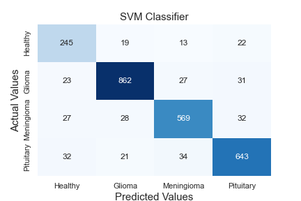
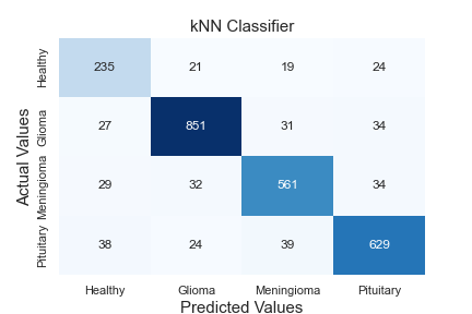
Thanks to the hidden layers in each classifier, features are extracted, and these extracted features are learned. The neurons in the output layer end the algorithm by labelling using the texture and edge features from the data sent to the classifier as input. While the first classifier contains two tag information, the second contains three. A comprehensive comparative analysis of the model against standard algorithms is shown in Table 9. A comparison of the method proposed in this article against existing models is made using different metrics. The proposed hybrid Elmann-BiLSTM model achieves better accuracy, precision, recall, and F-score than other classical machine and deep learning approaches. The first classifier makes the diseased-healthy classification. Remarkably, the tumour region's segmentation directly affects this classification's accuracy. Long Short Term Memory Algorithm (LSTM), k-Nearest Neighbor Algorithm (kNN), Support Vector Machine Algorithm (SVM), Random Forest Algorithm (RF), Multi-layer Perceptron Algorithm (MLP), Decision Tree Algorithm (DT), and Gradient Boost Classifier Algorithm (GBC) tests were carried out using the data amplified by the VAE-GAN architecture combined using methods. Accuracy values of 92.960%, 86.606%, 88.242%, 91.095%, 93.569%, 92.656%, and 89.649% were reached, respectively. The proposed hybrid Elmann-BiLSTM architecture classifies 5.937%, 12.291%, 10.655%, 7.802%, 5.328%, 6.241%, and 9.248% higher accuracy than these algorithms, respectively.
Figure 5 shows the confusion matrix of the algorithms in Table 9. When the matrices are examined in detail, it is seen that the proposed hybrid Elmann-BiLSTM model is a better classifier model. In general, all models classify data of healthy subjects with high accuracy. The most important reason is the absence of hyperintense regions in MRI images. The proposed method has considerably higher accuracy in classifying each tumor in both the first and second classifier blocks than other classical methods used for testing. The most important feature of the proposed method is that it correctly separates the input features of the model. However, the BiLSTM architecture is capable of both forward and reverse trains. In this way, the architecture is superior to the classical LSTM.
Table 8. Performance metrics of the two steps hybrid Elmann-BiLSTM model with different data combinations
|
|
|
First Step Elmann-BiLSTM Classifier |
Second Step Elmann-BiLSTM Classifier |
|||||
|
|
Metrics |
Healthy |
Tumor |
Accuracy |
Glioma |
Meningioma |
Pituitary |
Accuracy |
|
A |
Recall |
85.000% |
97.686% |
96.685% |
91.737% |
89.058% |
87.158% |
89.546% |
|
Precision |
75.893% |
98.701% |
92.128% |
86.431% |
88.611% |
|||
|
F-Score |
80.189% |
98.191% |
91.932% |
87.725% |
87.879% |
|||
|
B |
Recall |
90.000% |
98.372% |
97.711% |
95.551% |
93.617% |
93.169% |
94.259% |
|
Precision |
82.569% |
99.136% |
95.754% |
92.492% |
93.939% |
|||
|
F-Score |
86.125% |
98.753% |
95.652% |
93.051% |
93.552% |
|||
|
C |
Recall |
100% |
100% |
100% |
97.879% |
97.104% |
97.617% |
97.596% |
|
Precision |
100% |
100% |
98.611% |
97.104% |
96.744% |
|||
|
F-Score |
100% |
100% |
98.244% |
97.104% |
97.178% |
|||
|
D |
Recall |
100% |
100% |
100% |
99.576% |
98.933% |
99.315% |
99.313% |
|
Precision |
100% |
100% |
99.576% |
99.540% |
98.774% |
|||
|
F-Score |
100% |
100% |
99.576% |
99.236% |
99.044% |
|||
A: data augmentation techniques are not used, B: only classical data augmentation technique is used, C: only developed combined VAE-GAN data augmentation technique is used, D: both classical data augmentation technique and unified VAE-GAN data augmentation technique are used
Table 9. Comparison of the data produced by the proposed data expansion method VAE-GAN architecture and the performance of the proposed hybrid Elmann-BiLSTM classifier against different algorithms using different metrics
|
Algorithm |
Precision |
F-Score |
Recall |
Accuracy |
|
MLP |
93.567% |
93.568% |
93.569% |
93.569% |
|
SVM |
88.407% |
88.303% |
88.242% |
88.242% |
|
kNN |
86.810% |
86.685% |
86.606% |
86.606% |
|
RF |
91.084% |
91.088% |
91.095% |
91.095% |
|
DT |
92.666% |
92.657% |
92.656% |
92.656% |
|
GBC |
89.687% |
89.661% |
89.649% |
89.649% |
|
LSTM |
93.009% |
92.970% |
92.960% |
92.960% |
|
Proposed |
98.897% |
98.897% |
98.897% |
98.897% |
(a)
(b)
(c)
(d)
(e)
(f)
(g)
Figure 5. Confusion matrices of algorithms used for comparison. a: MLP, b: SVM, c: kNN, d: RF, e: DT, f: GBC, g: LSTM
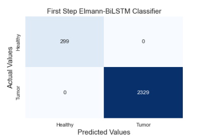
The matrix in which metrics such as precision and recall, frequently used in classification algorithms, are obtained is called the confusion matrix. The confusion matrix gives information about how accurately the classifier classifies which class. It also gives us clues about situations that cause confusion between classes. Figure 6 shows the complexity matrices of the proposed method. The algorithm has been tested both as a two-step classifier, as suggested and as a one-step classifier.
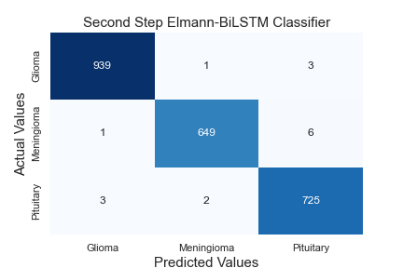
Figure 6(a) and 6(b) show the complexity matrix of the first and second classifier of the two-step classifier, respectively. When the complexity matrix of the first classifier is examined, it correctly predicts all 299 healthy data and 2329 tumor data. The second classifier uses data that the first classifier classifies as tumorous. Therefore, it uses a total of 2329 data for testing. The second classifier correctly predicted 939 of the 943 glioma images from these test data. He misclassified 1 data as meningioma and 3 data as pituitary. The second classifier correctly predicted 649 of the 656 meningioma images from these test data. He misclassified 1 data as glioma and 6 data as pituitary. The second classifier correctly predicted 725 of 730 pituitary images from these test data. Misclassified 2 data as meningioma and 3 data as glioma. Figure 6(c) is shown to examine the prediction performance that would be performed if the proposed model was a one-step classifier. In this test, the same data with the two-step classifier were used for the test. The one-step classifier correctly predicted 935 of the 943 glioma images from these test data. He misclassified 5 data as meningioma and 3 data as pituitary. The one-step classifier correctly predicted 647 of 656 meningioma images from these test data. He misclassified 2 data as glioma and 7 data as pituitary. The one-step classifier correctly predicted 718 of the 730 pituitary images from these test data. He misclassified 7 data as meningioma and 5 data as glioma. The one-step classifier also predicts all 299 healthy person data correctly. The main reason why both models accurately predict the data of healthy people is that the skull is stripped from the images, and the density difference is used in the segmentation process. However, due to the increase in the number of classes in the one-step classifier, the overall accuracy rate was 98.897%. It is also seen from the test results that using a two-step classifier increases the accuracy rate.
Table 10. Comparison of proposed methodology results for previous research studies
|
# |
Year |
Dataset |
Method |
Overall Accuracy |
|
[52] |
2018 |
[45] |
It proposes to use the KE-CNN algorithm for brain tumor classification without applying any segmentation process. |
Acc.: 93.68% |
|
[44] |
2018 |
[45] |
For brain tumor classification, the specialist performs segmentation (ROI-based). It also applies feature selection using 2D-DWT and 2D-Gabor filters. |
Acc.: 91.9% |
|
[39] |
2018 |
989 images |
Feature extraction was done using the CNN algorithm. Extracted features are used in DenseNet-LSTM architecture. |
Acc.: 92.13% |
|
[53] |
2018 |
Radiopedia |
It proposes a segmentation method on MR images using K-Means and Fuzzy C-Means methods. |
Acc.: 91.94% |
|
[54] |
2019 |
[45] |
After segmentation using Boundary Box, MR images were classified using Capsule Network architecture. |
Acc.: 90.89% |
|
[35] |
2019 |
[45] |
After noise reduction, contrast enhancement and edge detection pre-processing, MR images were classified by SVM algorithm. |
Acc.: 86.0% |
|
[55] |
2019 |
[45] |
After training the GAN architecture, it uses it as a classifier. In addition, 5-Fold cross-validation is used. |
Acc.: 95.6% |
|
[56] |
2019 |
BRATS 2015 |
After skull stripping, morphological operation, and normalization processes, classification was made using Enhanced CNN + BAT Algorithms. |
Prec: 87.0% Recall: 90.0% Acc.: 92.0% |
|
[57] |
2020 |
[45] |
Bayesian CapsNet architecture, a different approach for classification, is recommended for classification. |
Acc.: 73.9% |
|
[38] |
2020 |
[45] |
In the study, classification by SVM method is advocated after the steps of normalization, dense speeded-up robust features, and histogram of gradient approaches to ameliorate MRI quality and generate a discriminative feature set. |
Acc.: 94.7% |
|
[58] |
2021 |
[45] |
Classifying MR images with CapsNet architecture is recommended by applying 5-fold cross-validation. |
Acc.: 94.74% |
|
[59] |
2021 |
[45] |
It classifies MR images with EfficientNet-B0 architecture by applying Bounding Box and 5-fold cross-validation. |
Acc.: 98.04% |
|
[60] |
2022 |
[45] |
Classification of MR images with the EfficientNet-B0 and ResNet50 architectures is advocated by applying Bounding Box and 5-fold cross-validation. |
Acc.: 98.95% |
|
|
2022 |
Proposed Method |
In this proposed approach, tumor classification with the Hybrid Elmann-BiLSTM algorithm is proposed using synthetic MR images produced with the combined VAE-GAN architecture. |
Single Step: Acc.: 98.897% 2-Step: Acc. 1: 100% Acc. 2: 99.313% |
Acc.: Accuracy, Prec.: Precision
(a)
(b)
(c)
Figure 6. Confusion matrices of the hybrid Elmann-BiLSTM algorithm using data generated with the proposed unified VAE-GAN architecture
(a: confusion matrix of first step hybrid classifier, b: confusion matrix of second step hybrid classifier, c: confusion matrix of single step hybrid classifier)
(a) (b)
(c) (d)
Figure 7. Validation-accuracy and validation-loss graphs according to test results
(a: Validation-Accuracy graph of first step hybrid classifier, b: Validation-Loss graph of first step hybrid classifier, c: Validation-Accuracy graph of second step hybrid classifier, d: Validation-Loss graph of second step hybrid classifier)
Figure 7 shows the validation-accuracy and validation-loss graphs. According to iterations, the accuracy is almost 100%. When Figure 7(a) is examined, the precision value becomes almost 100% after a point. The highest precision value reached during the test phase is 100%, and the lowest is 96.744%. The validation-loss chart is shown in Figure 7(b). When the graph is examined, it is seen that the loss value is almost zero after a certain point. Figure 7(c) and 7(d) graphs are validation-accuracy and validation-loss graphs of the second classification block. A graph similar to the first classifier is obtained. In general, it is seen that the proposed Elmann-BiLSTM and combined VAE-GAN architecture achieves high accuracy both in data augmentation, segmentation and classification. Since most of the studies in Table 10 did not apply a data augmentation strategy, the overall accuracy rates are lower. It produces very successful results in data replication of VAE-GAN architecture. In addition, a solution has been created for the over-fitting problem of the model. It is also seen that the segmentation and feature extraction process against different types of tumors directly increases the accuracy. The effect of the density of the MRI images used in the segmentation process is eliminated with this proposed approach, and the model performs a more efficient segmentation process.
Tumor segmentation improves classification accuracy and reveals information about tumor size for radiotherapy and tumor surgery clinicians. In this way, an appropriate treatment plan can be made. A machine learning-based feature selection algorithm was used to eliminate the dimensionality problem of the features extracted with IGWT after segmentation, increasing the efficiency of both training and testing time. This reduces the computation time. The feature selection algorithm improves accuracy along with efficiency. In addition, the hybridization of the classification model also increases classification accuracy. The limited accuracy problem encountered in multiple classification studies was somewhat overcome with the hybrid approach. The BiLSTM architecture combined with the Elmann RNN architecture trains both forward and backward, thus improving the ability to distinguish features. In the studies encountered in the literature, a single-layer multi-classifier is generally used. This affects overall success. Therefore, this study proposes a two-layered classifier approach, achieving 100% accuracy in patient-healthy classification. In tumor classification, the accuracy is 99.313%. When the hybrid Elmann-BiLSTM model combined with the proposed VAE-GAN is compared with the studies carried out in the last five years in the literature (Table 10), it is seen that the accuracy performance of the model is relatively high. In the proposed approach, both the VAE-GAN data augmentation approach and the classifying Elmann-BiLSTM architecture increase the accuracy rate together.
This article proposes a framework that performs two-step classification with hybrid Elmann-BiLSTM architecture after dataset augmentation with unified VAE-GAN architecture. The algorithm is terminated if there is no tumor in the input data. If there is a tumor, the tumors are divided into three classes as glioma, meningioma and pituitary. Thanks to the proposed approach, a system that supports the decision-making of deep learning-based clinicians is designed with high accuracy. The dataset was augmented by combining decoder-encoder network and GAN architecture to solve the difficulty of obtaining medical images. The mode collapse problem encountered in the GAN architecture has been resolved with the VAE structure. The features were extracted with the IGWT method. However, the use of all features has an effect that will both reduce performance and prolong the processing time. A Binary Random Forest-based feature selection algorithm is used to prevent this and reduce dimensionality problems. A two-step classification is performed. The model created by hybridizing Elmann RNN architecture and BiLSTM architecture is used in both classifier blocks. The first classifier classifies only sick and healthy. If the classifier's result is healthy, it is concluded before the second classifier starts. The data is moved to the second classifier if the classifier's result is unhealthy. This classifier performs classification according to tumor type. The result of this classification is glioma, meningioma and pituitary.
Two publicly available datasets were used to evaluate the proposed model. As a result of the tests, the accuracy of the LSTM architecture, which is one of the classical approaches, is 92.960%. The accuracy of this proposed framework is 98.897% for the one-step classifier and 100% and 99.313% for the two-step classifier, respectively. It has been proven that this framework, proposed in line with the results obtained through the tests, can be used as a clinical decision support system for clinicians and neurologists. Results were compared with studies performed using the same dataset. In addition, the framework designed for future studies can be trained for different datasets and used to detect various diseases. In addition, tumor stage determination can be made using data with tumor stages information.
[1] Ismael, S.A.A., Mohammed, A., Hefny, H. (2020). An enhanced deep learning approach for brain cancer MRI images classification using residual networks. Artificial İntelligence in Medicine, 102: 101779. https://doi.org/10.1016/j.artmed.2019.101779
[2] Alther, B., Mylius, V., Weller, M., Gantenbein, A.R. (2020). From first symptoms to diagnosis: Initial clinical presentation of primary brain tumors. Clinical and Translational Neuroscience, 4(2): 2514183X20968368. https://doi.org/10.1177/2514183X20968368
[3] Lockman, P.R., Mittapalli, R.K., Taskar, K.S., Rudraraju, V., Gril, B., Bohn, K.A., Adkins, C.E., Roberts, A., Thorsheim, H.R., Gaasch, J.A., Huang, S., Palmieri, D., Steeg, P.S., Smith, Q.R. (2010). Heterogeneous blood–tumor barrier permeability determines drug efficacy in experimental brain metastases of breast cancer. Clinical Cancer Research, 16(23): 5664-5678. https://doi.org/10.1158/1078-0432.CCR-10-1564
[4] Lah, T.T., Novak, M., Breznik, B. (2020). Brain malignancies: Glioblastoma and brain metastases. Seminars in Cancer Biology, 60: 262-273. https://doi.org/10.1016/j.semcancer.2019.10.010
[5] Somasundaram, S., Gobinath, R. (2019). Current trends on deep learning models for brain tumor segmentation and detection–a review. In 2019 International Conference on Machine Learning, Big Data, Cloud and Parallel Computing (COMITCon), Faridabad, India, pp. 217-221. https://doi.org/10.1109/COMITCon.2019.8862209
[6] Pereira, S., Pinto, A., Alves, V., Silva, C.A. (2016). Brain tumor segmentation using convolutional neural networks in MRI images. IEEE Transactions on Medical İmaging, 35(5): 1240-1251. https://doi.org/10.1109/TMI.2016.2538465
[7] Kheifets, L., Repacholi, M., Saunders, R., Van Deventer, E. (2005). The sensitivity of children to electromagnetic fields. Pediatrics, 116(2): e303-e313. https://doi.org/10.1542/peds.2004-2541
[8] Wang, Y., Springer, S., Zhang, M., et al. (2015). Detection of tumor-derived DNA in cerebrospinal fluid of patients with primary tumors of the brain and spinal cord. Proceedings of the National Academy of Sciences, 112(31): 9704-9709. https://doi.org/10.1073/pnas.1511694112
[9] Amin, J., Sharif, M., Gul, N., Yasmin, M., Shad, S.A. (2020). Brain tumor classification based on DWT fusion of MRI sequences using convolutional neural network. Pattern Recognition Letters, 129: 115-122. https://doi.org/10.1016/j.patrec.2019.11.016
[10] Gyawali, S., Sharma, P., Mahapatra, A. (2019). Meningioma and psychiatric symptoms: An individual patient data analysis. Asian Journal of Psychiatry, 42: 94-103. https://doi.org/10.1016/j.ajp.2019.03.029
[11] McFaline-Figueroa, J.R., Lee, E.Q. (2018). Brain tumors. The American Journal of Medicine, 131(8): 874-882. https://doi.org/10.1016/j.amjmed.2017.12.039
[12] Tong, S., Wang, Y., Wu, J., Long, J., Zhong, P., Wang, B. (2021). Comprehensive pharmacogenomics characterization of temozolomide response in gliomas. European Journal of Pharmacology, 912: 174580. https://doi.org/10.1016/j.ejphar.2021.174580
[13] Zhang, L., Ren, Z. (2020). Comparison of CT and MRI images for the prediction of soft-tissue sarcoma grading and lung metastasis via a convolutional neural networks model. Clinical Radiology, 75(1): 64-69. https://doi.org/10.1016/j.crad.2019.08.008
[14] Langen, K.J., Galldiks, N., Hattingen, E., Shah, N.J. (2017). Advances in neuro-oncology imaging. Nature Reviews Neurology, 13(5): 279-289. https://doi.org/10.1038/nrneurol.2017.44
[15] Rosen, J., Stoffels, G., Lohmann, P., Bauer, E.K., Werner, J.M., Wollring, M., Rapp, M., Felsberg, J., Kocher, M., Fink, G.R., Langen, K., Galldiks, N. (2021). Prognostic value of pre-irradiation FET PET in patients with not completely resectable IDH-wildtype glioma and minimal or absent contrast enhancement. Scientific Reports, 11(1): 1-9. https://doi.org/10.1038/s41598-021-00193-x
[16] Makino, Y., Arakawa, Y., Yoshioka, E., Shofuda, T., Kawauchi, T., Terada, Y., Tanji, M., Kanematsu, D., Mineharu, Y., Miyamoto, S., Kanemura, Y. (2021). Prognostic stratification for IDH-wild-type lower-grade astrocytoma by Sanger sequencing and copy-number alteration analysis with MLPA. Scientific Reports, 11(1): 1-12. https://doi.org/10.1038/s41598-021-93937-8
[17] Izquierdo, C., Barritault, M., Poncet, D., Cartalat, S., Joubert, B., Bruna, J., Jouanneau, E., Guyotat, J., Vasiljevic, A., Fenouil, T., Berthezène, Y., Honnorat, J., Meyronet, D., Ducray, F. (2019). Radiological characteristics and natural history of adult IDH-wildtype astrocytomas with TERT promoter mutations. Neurosurgery, 85(3): E448-E456. https://doi.org/10.1093/neuros/nyy513
[18] Alwadani, B., Dall’Angelo, S., Fleming, I.N. (2021). Clinical value of 3'-deoxy-3'-[18F] fluorothymidine-positron emission tomography for diagnosis, staging and assessing therapy response in lung cancer. Insights into Imaging, 12(1): 1-21. https://doi.org/10.1186/s13244-021-01026-1
[19] Song, S., Cheng, Y., Ma, J., Wang, L., Dong, C., Wei, Y., Xu, G., An, Y., Qi, Z., Lin, Q., Lu, J. (2020). Simultaneous FET-PET and contrast-enhanced MRI based on hybrid PET/MR improves delineation of tumor spatial biodistribution in gliomas: A biopsy validation study. European Journal of Nuclear Medicine and Molecular İmaging, 47(6): 1458-1467. https://doi.org/10.1007/s00259-019-04656-2
[20] Lohmann, P., Stavrinou, P., Lipke, K., Bauer, E.K., Ceccon, G., Werner, J.M., Neumaier, B., Fink, G.R., Shah, N.J., Langen, K., Galldiks, N. (2019). FET PET reveals considerable spatial differences in tumour burden compared to conventional MRI in newly diagnosed glioblastoma. European Journal of Nuclear Medicine and Molecular İmaging, 46(3): 591-602. https://doi.org/10.1007/s00259-018-4188-8
[21] Ghaffari, M., Sowmya, A., Oliver, R. (2019). Automated brain tumor segmentation using multimodal brain scans: A survey based on models submitted to the BraTS 2012–2018 challenges. IEEE Reviews in Biomedical Engineering, 13: 156-168. https://doi.org/10.1109/RBME.2019.2946868
[22] Badža, M.M., Barjaktarović, M.Č. (2020). Classification of brain tumors from MRI images using a convolutional neural network. Applied Sciences, 10(6): 1999. https://doi.org/10.3390/app10061999
[23] Eom, J.H., Kim, S.C., Zhang, B.T. (2008). AptaCDSS-E: A classifier ensemble-based clinical decision support system for cardiovascular disease level prediction. Expert Systems with Applications, 34(4): 2465-2479. https://doi.org/10.1016/j.eswa.2007.04.015
[24] Varuna Shree, N., Kumar, T.N.R. (2018). Identification and classification of brain tumor MRI images with feature extraction using DWT and probabilistic neural network. Brain İnformatics, 5(1): 23-30. https://doi.org/10.1007/s40708-017-0075-5
[25] Komatsu, M., Sakai, A., Dozen, A., Shozu, K., Yasutomi, S., Machino, H., Asada, K., Kaneko, S., Hamamoto, R. (2021). Towards clinical application of artificial intelligence in ultrasound imaging. Biomedicines, 9(7): 720. https://doi.org/10.3390/biomedicines9070720
[26] Chien, C.Y., Hsu, S.W., Lee, T.L., Sung, P.S., Lin, C.C. (2020). Using artificial neural network to discriminate Parkinson’s disease from other Parkinsonisms by focusing on putamen of dopamine transporter SPECT images. Biomedicines, 9(1): 12. https://doi.org/10.3390/biomedicines9010012
[27] Moreau, G., François-Lavet, V., Desbordes, P., Macq, B. (2021). Reinforcement learning for radiotherapy dose fractioning automation. Biomedicines, 9(2): 214. https://doi.org/10.3390/biomedicines9020214
[28] Lee, C.C., Lee, W.K., Wu, C.C., Lu, C.F., Yang, H.C., Chen, Y.W., Chung, W.Y., Hu, Y.S., Wu, H.M., Wu, Y.T., Guo, W.Y. (2021). Applying artificial intelligence to longitudinal imaging analysis of vestibular schwannoma following radiosurgery. Scientific Reports, 11(1): 1-10. https://doi.org/10.1038/s41598-021-82665-8
[29] Ding, L., Fang, W., Luo, H., Love, P.E., Zhong, B., Ouyang, X. (2018). A deep hybrid learning model to detect unsafe behavior: Integrating convolution neural networks and long short-term memory. Automation in Construction, 86: 118-124. https://doi.org/10.1016/j.autcon.2017.11.002
[30] Yang, H., Sun, J., Carass, A., Zhao, C., Lee, J., Xu, Z., Prince, J. (2018). Unpaired brain MR-to-CT synthesis using a structure-constrained CycleGAN. In: Stoyanov, D., et al. (eds) Deep Learning in Medical Image Analysis and Multimodal Learning for Clinical Decision Support. DLMIA ML-CDS 2018 2018. Lecture Notes in Computer Science(), vol 11045. Springer, Cham. https://doi.org/10.1007/978-3-030-00889-5_20
[31] Goodfellow, I., Pouget-Abadie, J., Mirza, M., Xu, B., Warde-Farley, D., Ozair, S., Courville, A., Bengio, Y. (2020). Generative adversarial networks. Communications of the ACM, 63(11): 139-144. https://doi.org/10.1145/3422622
[32] Wu, X., Bi, L., Fulham, M., Feng, D.D., Zhou, L., Kim, J. (2021). Unsupervised brain tumor segmentation using a symmetric-driven adversarial network. Neurocomputing, 455: 242-254. https://doi.org/10.1016/j.neucom.2021.05.073
[33] Cirillo, M. D., Abramian, D., Eklund, A. (2020). Vox2Vox: 3D-GAN for brain tumour segmentation. In: Crimi, A., Bakas, S. (eds) Brainlesion: Glioma, Multiple Sclerosis, Stroke and Traumatic Brain Injuries. BrainLes 2020. Lecture Notes in Computer Science(), vol 12658. Springer, Cham. https://doi.org/10.1007/978-3-030-72084-1_25
[34] Jiang, M., Zhi, M., Wei, L., Yang, X., Zhang, J., Li, Y., Wang, P., Huang, J., Yang, G. (2021). FA-GAN: Fused attentive generative adversarial networks for MRI image super-resolution. Computerized Medical Imaging and Graphics, 92: 101969. https://doi.org/10.1016/j.compmedimag.2021.101969
[35] Tahir, B., Iqbal, S., Usman Ghani Khan, M., Saba, T., Mehmood, Z., Anjum, A., Mahmood, T. (2019). Feature enhancement framework for brain tumor segmentation and classification. Microscopy Research and Technique, 82(6): 803-811. https://doi.org/10.1002/jemt.23224
[36] Liu, Y., Chen, A., Shi, H., Huang, S., Zheng, W., Liu, Z., Zhang, Q., Yang, X. (2021). CT synthesis from MRI using multi-cycle GAN for head-and-neck radiation therapy. Computerized Medical Imaging and Graphics, 91: 101953. https://doi.org/10.1016/j.compmedimag.2021.101953
[37] Nguyen, H.T., Le, T.T., Nguyen, T.V., Nguyen, N.T. (2020). Enhancing MRI brain tumor segmentation with an additional classification network. In: Crimi, A., Bakas, S. (eds) Brainlesion: Glioma, Multiple Sclerosis, Stroke and Traumatic Brain Injuries. BrainLes 2020. Lecture Notes in Computer Science(), vol 12658. Springer, Cham. https://doi.org/10.1007/978-3-030-72084-1_45
[38] Ayadi, W., Charfi, I., Elhamzi, W., Atri, M. (2020). Brain tumor classification based on hybrid approach. The Visual Computer, 38: 107-117. https://doi.org/10.1007/s00371-020-02005-1
[39] Zhou, Y., Li, Z., Zhu, H., Chen, C., Gao, M., Xu, K., Xu, J. (2018). Holistic brain tumor screening and classification based on densenet and recurrent neural network. In: Crimi, A., Bakas, S., Kuijf, H., Keyvan, F., Reyes, M., van Walsum, T. (eds) Brainlesion: Glioma, Multiple Sclerosis, Stroke and Traumatic Brain Injuries. BrainLes 2018. Lecture Notes in Computer Science(), vol 11383. Springer, Cham. https://doi.org/10.1007/978-3-030-11723-8_21
[40] Paul, J.S., Plassard, A.J., Landman, B.A., Fabbri, D. (2017). Deep learning for brain tumor classification. In Medical Imaging 2017: Biomedical Applications in Molecular, Structural, and Functional Imaging, 10137: 253-268. https://doi.org/10.1117/12.2254195
[41] Abiwinanda, N., Hanif, M., Hesaputra, S.T., Handayani, A., Mengko, T.R. (2019). Brain tumor classification using convolutional neural network. In: Lhotska, L., Sukupova, L., Lacković, I., Ibbott, G.S. (eds) World Congress on Medical Physics and Biomedical Engineering 2018. IFMBE Proceedings, vol 68/1. Springer, Singapore. https://doi.org/10.1007/978-981-10-9035-6_33
[42] Ge, C., Gu, I.Y.H., Jakola, A.S., Yang, J. (2018). Deep learning and multi-sensor fusion for glioma classification using multistream 2D convolutional networks. In 2018 40th Annual International Conference of the IEEE Engineering in Medicine and Biology Society (EMBC), Honolulu, HI, USA, pp. 5894-5897. https://doi.org/10.1109/EMBC.2018.8513556
[43] Rehman, A., Naz, S., Razzak, M. I., Akram, F., Imran, M. (2020). A deep learning-based framework for automatic brain tumors classification using transfer learning. Circuits, Systems, and Signal Processing, 39(2): 757-775. https://doi.org/10.1007/s00034-019-01246-3
[44] Ismael, M.R., Abdel-Qader, I. (2018). Brain tumor classification via statistical features and back-propagation neural network. In 2018 IEEE İnternational Conference on Electro/İnformation Technology (EIT), Rochester, MI, USA, pp. 0252-0257. https://doi.org/10.1109/EIT.2018.8500308
[45] Cheng, J., Huang, W., Cao, S., Yang, R., Yang, W., Yun, Z., Wang, Z., Feng, Q. (2015). Enhanced performance of brain tumor classification via tumor region augmentation and partition. PloS One, 10(10): e0140381. https://doi.org/10.1371/journal.pone.0140381
[46] Sartaj Bhuvaji, Ankita Kadam, Prajakta Bhumkar, Sameer Dedge and Swati Kanchan. (2020)., Brain Tumor Classification (MRI) [Dataset]. Kaggle. https://doi.org/10.34740/KAGGLE/DSV/1183165
[47] Caraffa, L., Tarel, J.P., Charbonnier, P. (2015). The guided bilateral filter: When the joint/cross bilateral filter becomes robust. IEEE Transactions on Image Processing, 24(4): 1199-1208. https://doi.org/10.1109/TIP.2015.2389617
[48] Shanthini, A., Manogaran, G., Vadivu, G., Kottilingam, K., Nithyakani, P., Fancy, C. (2021). Threshold segmentation based multi-layer analysis for detecting diabetic retinopathy using convolution neural network. Journal of Ambient Intelligence and Humanized Computing, 1-15. https://doi.org/10.1007/s12652-021-02923-5
[49] Breiman, L. (2001). Random forests. Machine Learning, 45(1): 5-32. https://doi.org/10.1023/A:1010933404324
[50] Li, J., Cheng, K., Wang, S., Morstatter, F., Trevino, R.P., Tang, J., Liu, H. (2017). Feature selection: A data perspective. ACM Computing Surveys (CSUR), 50(6): 1-45. https://doi.org/10.1145/3136625
[51] Gurumurthy, S., Kiran Sarvadevabhatla, R., Venkatesh Babu, R. (2017). DeLiGAN: Generative adversarial networks for diverse and limited data. In 2017 IEEE Conference on Computer Vision and Pattern Recognition (CVPR), Honolulu, HI, USA, pp. 4941-4949. https://doi.org/10.1109/CVPR.2017.525
[52] Pashaei, A., Sajedi, H., Jazayeri, N. (2018). Brain tumor classification via convolutional neural network and extreme learning machines. In 2018 8th International Conference on Computer and Knowledge Engineering (ICCKE), Mashhad, Iran, pp. 314-319. https://doi.org/10.1109/ICCKE.2018.8566571
[53] Almahfud, M.A., Setyawan, R., Sari, C.A., Rachmawanto, E.H. (2018). An effective MRI brain image segmentation using joint clustering (K-Means and Fuzzy C-Means). In 2018 International Seminar on Research of Information Technology and Intelligent Systems (ISRITI), Yogyakarta, Indonesia, pp. 11-16. https://doi.org/10.1109/ISRITI.2018.8864326
[54] Afshar, P., Plataniotis, K.N., Mohammadi, A. (2019). Capsule networks for brain tumor classification based on MRI images and coarse tumor boundaries. In ICASSP 2019-2019 IEEE International Conference on Acoustics, Speech and Signal Processing (ICASSP), Brighton, UK, pp. 1368-1372. https://doi.org/10.1109/ICASSP.2019.8683759
[55] Ghassemi, N., Shoeibi, A., Rouhani, M. (2020). Deep neural network with generative adversarial networks pre-training for brain tumor classification based on MR images. Biomedical Signal Processing and Control, 57: 101678. https://doi.org/10.1016/j.bspc.2019.101678
[56] Thaha, M.M., Kumar, K., Murugan, B.S., Dhanasekeran, S., Vijayakarthick, P., Selvi, A.S. (2019). Brain tumor segmentation using convolutional neural networks in MRI images. Journal of Medical Systems, 43(9): 1-10. https://doi.org/10.1007/s10916-019-1416-0
[57] Afshar, P., Mohammadi, A., Plataniotis, K.N. (2020). BayesCap: A Bayesian approach to brain tumor classification using capsule networks. IEEE Signal Processing Letters, 27: 2024-2028. https://doi.org/10.1109/LSP.2020.3034858
[58] Ayadi, W., Elhamzi, W., Charfi, I., Atri, M. (2021). Deep CNN for brain tumor classification. Neural Processing Letters, 53(1): 671-700. https://doi.org/10.1007/s11063-020-10398-2
[59] Guan, Y., Aamir, M., Rahman, Z., Ali, A., Abro, W.A., Dayo, Z.A., Bhutta, M.S., Aamir, M., Hu, Z. (2021). A framework for efficient brain tumor classification using MRI images. Mathematical Biosciences and Engineering, 18(5): 5790-5815. https://doi.org/10.3934/MBE.2021292
[60] Aamir, M., Rahman, Z., Dayo, Z. A., Abro, W.A., Uddin, M.I., Khan, I., Imran, A.S., Ali, Z., Ishfaq, M., Guan, Y., Hu, Z. (2022). A deep learning approach for brain tumor classification using MRI images. Computers and Electrical Engineering, 101: 108105. https://doi.org/10.1016/j.compeleceng.2022.108105