Ting Shao![]() | Jing Xu
| Jing Xu![]() | Yaqin Dai*
| Yaqin Dai*![]()
© 2024 The authors. This article is published by IIETA and is licensed under the CC BY 4.0 license (http://creativecommons.org/licenses/by/4.0/).
OPEN ACCESS
This study explores the feasibility and application value of the Faster R-CNN algorithm, a deep learning technology, in identifying signal abnormalities and locating injury areas in MRI images of the spinal cord. Method: Initially, Magnetic Resonance Imaging (MRI) images from 1,000 spinal cord injury (SCI) patients and 500 healthy individuals collected over five years were included in the dataset, divided into signal change and normal groups. The dataset was then preprocessed, and the lesion areas were annotated by experienced spine surgeons for later experimental verification of the algorithm's effectiveness; no markings were necessary for the normal group. Subsequently, the Faster R-CNN algorithm, combined with the VGG-16 and Resnet50 network models from the convolutional neural network (CNN) framework, was used for recognizing and locating SCI in MRI images. Finally, a horizontal comparison of different network structure models was conducted, with the model's mean Average Precision (mAP) and visual results serving as evaluation metrics to determine the best network structure model. The deep learning model constructed in this paper can use real-time medical imaging of SCI patients as input for the spinal cord analysis neural network. The trained network can automatically identify and label the location of SCI, achieving a model mAP of 88.6% and an image test speed of 0.22s per image.
spinal cord injury (SCI), Magnetic Resonance Imaging (MRI), convolutional neural network (CNN), faster R-CNN, VGG-16, Resnet50
SCI is caused by various reasons leading to structural and functional damage to the spinal cord, resulting in partial or complete loss of motor, sensory, and autonomic nervous functions below the level of injury, primarily due to trauma [1-3]. There are nearly 40 million SCI patients worldwide, with over a million in China alone. The annual incidence rate is 37 per million, increasing by 120,000 each year [4, 5]. SCI not only causes structural and functional damage to the body but also leads to many complications. About 80% of patients suffer from neurogenic bladder and neurogenic bowel dysfunction [6, 7], have a significantly higher risk of venous thrombosis embolism (VTE) [8] and pressure injury (PI) [9] than the general population, and severe respiratory dysfunction has become the leading cause of death in the acute and chronic recovery phases [10]. Therefore, the high disability rate, mortality rate, complication rate, long rehabilitation time, and poor outcome of SCI severely affect the physical and mental health and quality of life of patients [11]. Since there is currently no effective cure for SCI, how to diagnose and differentiate the injury site for SCI patients as soon as possible, quickly clarify and implement treatment plans, reduce the incidence and disability rate of complications, restore bodily functions, and improve the survival quality of patients has always been the focus of SCI research.
MRI of the spine is one of the important means for diagnosing spinal diseases clinically. MRI is highly valuable in observing the shape of the spinal cord, signal intensity, vertebral bone quality, and changes in intervertebral discs [12], and provides clear indications of spinal cord edema and hemorrhage. It not only helps determine the cause and extent of neurological impairment, the possible mechanism of injury, and spinal instability but also provides important auxiliary reference for the diagnosis and differentiation of SCI. In recent years, deep learning technology has achieved good results in the field of medical image recognition, especially in disease detection and identification. For instance, Anantharajan et al. [13] used deep learning and machine learning methods combined with brain MRI images for brain tumor detection, Bousis et al. [14] conducted a survey of deep learning detection of skin cancer research results, organizing the most common deep learning models and datasets used for skin cancer classification, and Lundervold and Lundervold [15] studied the application of deep learning technology from MRI image acquisition to image retrieval, segmentation, and disease prediction. In recent years, more and more clinical departments have combined MRI image datasets with machine learning for the diagnosis and treatment of spinal cord diseases. For example, de Paiva et al. [16] reviewed the most common and noteworthy intramedullary and extramedullary spinal tumors, as well as other tumor mimetics, with a focus on their MRI morphological features. Zhang et al. [17] proposed that machine learning and PPI analysis can help screen and diagnose the basic PRG (pyroptosis related genes) for SCI. Kim et al. [18] developed an advanced predictive model for pressure ulcer occurrence in SCI patients using machine learning (ML) technology. Jazayeri et al. [19] uses machine learning algorithms to develop a region based prediction model for the incidence rate of traumatic spinal cord injury. However, due to the wide variability in the shape, length, and range of lesions of the spinal cord, and issues with image changes in size, resolution, orientation, contrast, and artifacts, their research application in large clinical studies of multi-part images has been limited. Currently, the application of deep learning technology in common spinal diseases on MRI images is relatively scarce. We attempt to use deep learning technology to preliminarily explore the location identification and detection of SCI on MRI images, which could further provide a possibility for its clinical application. With the continuous deepening of clinical research on SCI, there has been significant progress in the mechanisms and medications of SCI, but clinical research still remains at the primitive manual level, with diagnosis of SCI still based on experience and visual estimation, without quantification of the specific size of SCI or specific degree division of the same layer SCI signals. To address the problems in the existing technology, this paper collects MRI imaging data of SCI patients, gathers a dataset, and uses the deep learning technology—Faster R-CNN to recognize, detect, and locate lesions in SCI MRI images, and evaluates deep learning network models, comparing the prediction effects and detection speeds of different network architecture models, verifying the effectiveness of the big data + artificial intelligence model in the identification and detection of SCI diseases, laying a foundation for more extensive research in the field of spinal and spinal cord imaging in the future.
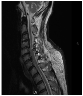
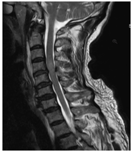
Typically, when spinal injuries involve the spinal cord, they can manifest as various degrees of signal changes. MRI can not only observe the morphological changes of acute SCI but can also precisely determine the degree of SCI based on changes in the spinal cord signal. Moreover, it can detect occult fractures and spinal cord edema, which significantly guides the formulation of treatment plans and the determination of prognosis. The MRI manifestations of SCI vary according to different lesion presentations. We consulted relevant literature on the MRI of SCI [20-22] and sought advice from professional spinal surgeons regarding its classification, finding two main types: one is based on the cause of injury, using cervical SCI as an example, which can be divided into Types I-IV, as shown in Figure 1 and Table 1; another classification method is based on the pathological changes in the spinal cord tissue, mainly divided into hemorrhage, edema, mixed type, etc., as shown in Table 2. From a medical professional perspective, the cause of injury in the first classification ultimately leads to pathological changes in the spinal cord that follow. For instance, cystic changes and glial scar formation, such types of pathological changes, usually occur during the recovery period, with early manifestations primarily being hemorrhage, edema, and mixed type. Therefore, this paper mainly uses the second classification method to detect the types of signal abnormalities in MRI and summarizes the characteristics of signal changes in SCI on MRI as shown in Table 2.
Figure 1. Imaging classification of acute cervical SCI (based on cause of injury)
Table 1. Imaging classification of acute cervical SCI (based on cause of injury)
|
Number |
Category |
Compression Factors |
Type of Injury |
|
A |
Type I |
Spinal cord under significant compression, mainly due to pathological changes in the cervical spine |
Congenital cervical spinal canal stenosis |
|
B |
Ossification of the posterior longitudinal ligament |
||
|
C |
Degenerative changes such as disc herniation, osteophyte formation at the vertebral edge, and ligamentum flavum hypertrophy |
||
|
D |
Type II |
Spinal cord under significant compression, mainly due to traumatic disc herniation or epidural hematoma |
Traumatic disc herniation |
|
E |
Epidural hematoma |
||
|
F |
Type III |
No significant spinal cord compression |
Presence of definitive signs of injury to the disc-ligament complex (DLC) |
|
G |
Type IV |
Absent or only suspicious signs of DLC injury |
Table 2. Types of MRI manifestations and signal changes in SCI (based on pathological changes in spinal cord tissue)
|
Number |
Type of Lesion |
MRI Signal Changes |
|
1 |
Hemorrhagic |
Slightly higher signal on T1WI, high signal on T2WI. If there is a large central low signal area on the spinal cord's T1-weighted image, it indicates gray matter hemorrhage. |
|
2 |
Edematous |
Low or iso signal on T1WI, high signal on T2WI. |
|
3 |
Mixed |
Presents mixed high and low uneven signals within the spinal cord. |
3.1 Data collection
(1) Dataset acquisition: The dataset consists of spinal cord MRI examination results of patients treated for SCI at our hospital from January 2018 to January 2023; a total of 1,000 patients, including 592 males and 418 females. The patient's age ranges from 13 to 70 years old, with an average of 41.8 years old. Traumatic spinal cord injury is the main cause, including car accidents, heavy object injuries, high-altitude falls, falls, and other injuries. Additionally, MRI scans from 500 healthy individuals (i.e., MRIs not diagnosed with SCI) were collected, totaling 1,500 individuals for the MRI image dataset.
(2) Data grouping: The collected radiological dataset was divided into two groups, the "normal group" and the "abnormal group," with 500 and 1,000 cases, respectively. Of these, 800 (about 80%) from the abnormal group were used as the training set, and the remaining 200 (about 20%) as the validation set. The inclusion criteria for the normal group are based on the doctor's diagnosis that MRI images do not show spinal cord injury, while the inclusion criteria for the abnormal group are based on the doctor's diagnosis that MRI images show varying degrees of spinal cord injury, including spinal cord gray matter hemorrhage, spinal cord edema with high signal intensity, cervical fracture and dislocation, combined with varying degrees of intervertebral disc herniation, combined with extraspinal hematoma and paravertebral soft tissue injury.
(3) Data security: Before collecting data, the research team obtained informed consent from all patients, informing them of the research purpose. To protect participants' privacy, the team anonymized the collected image data. Access to the data was restricted to team members involved in the research for processing and analysis purposes only.
3.2 Sample labeling and retrieval
Before conducting the experiment, the collected dataset needed to be preprocessed. First, two experienced spinal surgeons used LabelMe Toolbox-master software to annotate the lesion areas in the abnormal group for the training and validation sets to later verify the algorithm's effectiveness; the normal group was not marked. The annotation process used the LabelMe Toolbox-master tool for standard naming, framing the sample's name, size, location, etc., with bounding boxes and annotating image prompt information. The markings and annotations were saved in XML file format. As shown in Table 3, this indicates the annotated location of the lesion area for edematous SCI signal changes.
Table 3. Labeling of lesion areas for edematous SCI
|
Number |
Original Image |
Spinal Cord Abnormal Signal Label |
Annotation |
|
1 |
L4/5 significant disc herniation with free compression of the spinal cord, noticeable edema and high signal above the nucleus pressing on the spinal cord. |
||
|
2 |
Cervical spondylotic myelopathy, multi-segmental spinal canal stenosis, long-term compression of the spinal cord, MRI indicates local edema with high signal, significant behind the C5 vertebra. |
||
|
3 |
Cervical conus canal stenosis, C4/5, C5/6 disc herniation, high signal edema behind the 4th cervical vertebra in the spinal cord. |
3.3 Image preprocessing
To prevent overfitting in the learning process of visual tasks due to a small amount of data and to further improve the performance of the neural network model, reduce the model's sensitivity to images, and avoid sample imbalance [23], it is necessary to perform data augmentation on image data. First, batch processing is applied to the original MRI images to standardize all images to a size of 600*800, and label extraction is conducted to form an MRI image database. The normalization process uses formula (1) to adjust the image grayscale to the range of 0-255.
$G_1(x, y)=\left(G_0(x, y)-\min \left(G_0\right)\right) \times \frac{255-0}{\max \left(G_0\right)-\min \left(G_0\right)}$ (1)
Among them, G0(x,y) is the grayscale value of the original MRI image at (x, y) pixels, and G1(x,y) is the grayscale value of the digitized MRI image at (x, y) pixels after grayscale normalization. All subsequent operations are performed on grayscale normalized images G1(x,y).
Then, data augmentation, including angle rotation, horizontal flipping, vertical flipping, and random scaling, expands the data to 10 times its original size, with image specifications of 600*800 (length*width*RGB). The ImageDataGenerator module of Python's keras library [24] has several parameters for transforming images in different ways. This study mainly expanded the training set sample data through four methods, as shown in Table 4:
Table 4. Data augmentation methods and parameters
|
Parameter Name |
Parameter Setting |
Meaning |
|
rotation_range |
30 |
Images are randomly rotated between 0 and 30 degrees |
|
zoom_range |
0.2 |
Images are randomly scaled by 0.2, [lower, upper] = [0.8, 1.2] |
|
horizontal_flip |
true |
Images are randomly flipped horizontally |
|
vertical_flip |
true |
Images are randomly flipped vertically |
4.1 Detection steps
(1) Create an experimental dataset using MRI medical images containing SCI;
(2) Preprocess the experimental dataset and adjust parameters of the spinal cord analysis neural network to be trained;
(3) Input the preprocessed dataset into the to-be-trained spinal cord analysis neural network for model training, to obtain a trained spinal cord analysis neural network;
(4) Use real-time medical imaging of SCI patients as input to the trained spinal cord analysis neural network, to automatically detect and identify the SCI lesion area, and the coordinates and size of the SCI in the image.
4.2 Detection task
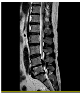
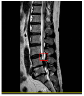
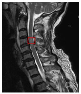
Our experimental task involves image recognition and target localization detection. First, input an MRI image, identify the target image with signal abnormalities in the image and output the category of signal abnormalities as shown in Table 2, and also mark the target object with a frame. Coordinate localization includes the upper left corner (x,y) coordinates of the "frame" as well as width and height, represented as (x,y,w,h), framing as shown in Figure 2.
Figure 2. Coordinate localization of signal abnormal areas
(a)
(b)
(c)
(d)
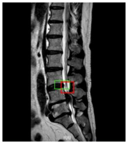
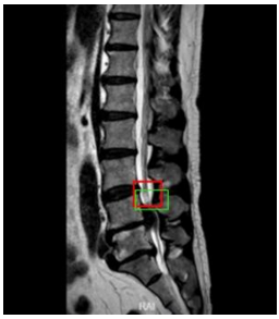
Figure 3. Overlap or ratio score between hypothetical and actual frames
The specific principles and steps of target localization are: 1) Set "frames" of different sizes; 2) Distribute these frames around the target image location, calculate the score for each frame; 3) Based on the scores, select the frame with the highest score. As shown in Figure 3, for a given image, frames of different sizes capture the image, and the captured frames with images are used as input for training and learning. After learning, the classification score of each frame and the corresponding regression position (x,y,w,h) are calculated and output. Then, the detection evaluation function used is the intersection-over-union (IOU) to select the best target frame, comparing the located frame with the actual position. The IOU is the result calculated by dividing the part of the intersection that overlaps between two regions by the union set part of the two regions, i.e., IOU=(prediction ∩ reality)/(predictionÈreality). IOU can be used to measure the task of outputting a predicted range (bounding boxes), and it measures the correlation between prediction and reality. The higher the correlation, the higher the ratio. In Figure 3, the red frame is the actual frame, and the green frame is the hypothetical frame. We expect a green frame to completely overlap with the red frame, but this is difficult to achieve in reality, leading to some overlap between various hypothetical frames and the actual frame, represented by IOU: (a) the green frame in the upper left corner scores 0.6; (b) the green frame in the upper right corner scores 0.8; (c) the green frame in the lower left corner scores 0.5; (d) the green frame in the lower right corner scores 0.75. When using IOU for object detection, the following steps are generally required: 1) Manually mark the target range of the object to be detected (ground-truth bounding boxes) in the training set images; 2) Obtain the predicted result range through the training algorithm.
5.1 Choice of feature extraction network
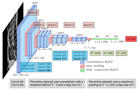
Figure 4. VGG-16 Network Structure
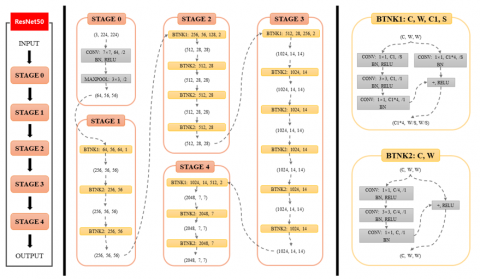
Figure 5. ResNet50 network structure and intermediate dimension transformation
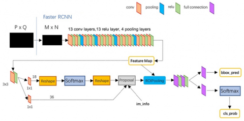
Figure 6. Faster R-CNN network structure
In recent years, CNNs have become representative of deep neural network models, with a network structure that shares weights, making it more biomimetic and thus reducing the complexity of the network model. This advantage is even more apparent when the network input is multi-dimensional images, to the extent that images can bypass the feature extraction and data reshaping processes of traditional algorithms and be directly used as network input. Based on the characteristics of the MRI dataset in this paper, the neural network experiment chooses VGG-16 [25] and Resnet50 [26] as the main frameworks for feature extraction. The VGG-16 network, which was trained on a database of a million images, has 16 layers deep. Its computational feature is the repeated stacking of small 3*3 convolutional kernels and 2*2 max pooling layers, with performance improvement achieved by deepening the network structure continuously. VGGNet has good scalability and extensibility, and its generalization on other image data applications is excellent. Below, Figure 4 shows the VGG-16 network structure.
The Residual Network (ResNet), proposed in 2015, won first place in the ImageNet competition classification task. Its main advantage lies in its simplicity and practicality. For example, ResNet models are used in areas such as image detection, segmentation, and recognition. Papers [27, 28] and other research results have confirmed the practicality and effectiveness of ResNet. Therefore, another CNN model we use in our experiment is ResNet50. The characteristic of the ResNet50 network structure is that it introduces Batch Normalization (BN) layers and abandons Dropout to solve the problems of gradient disappearance and explosion. At the same time, it introduces residuals to solve the problem of network degradation. The network structure of ResNet50 and the intermediate dimension transformation are shown in Figure 5.
5.2 Object detection and localization algorithm selection
In recent years, various object detection technologies have rapidly evolved. Fast R-CNN, building on the foundation of R-CNN, adopted the SPP Net method for improvements that significantly enhanced computational performance. The Faster RCNN algorithm [29] introduced the Region Proposal Network (RPN) candidate box generation algorithm on top of Fast R-CNN, integrating feature extraction, proposal extraction, bounding box regression (rectrefine), and classification into one network, thus significantly improving overall performance, particularly in terms of detection speed. As shown in Figure 6 below, Faster R-CNN consists of the following parts: (1) Dataset, image input; (2) Convolutional layer CNN and other base networks, to extract features and obtain a feature map; (3) RPN layer, which uses a 3*3 slide window on the feature map extracted by the convolutional layer to traverse the entire feature map. In this process, each window center generates 9 anchors at different rates and scales (1:2, 1:1, 2:1). Then, it uses a fully connected layer to perform binary classification (foreground or background) for each anchor and preliminary b-box regression, finally outputting approximately 300 precise ROIs. (4) The feature map from the convolutional layer is fixed to the input dimension of the fully connected layer using ROI pooling. (5) The ROIs outputted by the RPN are then mapped onto the feature map in ROI pooling to perform b-box regression and classification.
5.3 Network initialization and tuning
Our experiment employs the Faster R-CNN algorithm, based on the VGG16 and ResNet50 CNNs, for detecting disc herniation, lesions, or signal abnormalities in spinal MRI. Before model training, the network is initialized and tuned as follows: (a) Algorithm adoption strategy: The target detection framework uses the Faster R-CNN framework. CNNs or their derivative networks often serve as the basic backbone for other complex networks. This experiment used the VGG-16 and ResNet-50 network models, which have also been initialized for training to achieve better training effects. (b) Perform end-to-end training of RPN, where the network uses the ImageNet pre-trained model for initialization. (c) Use the proposal regions generated by RPN in step two to train Fast R-CNN, also using the ImageNet pre-trained model for model initialization. (d) Use the parameters from the previous step's Fast R-CNN to initialize RPN, fix the convolutional base layer, and only fine-tune the layers unique to RPN (the convolutional layers are shared at this step). (e) Fix the convolutional base layer and only fine-tune the layers unique to Fast R-CNN.
5.4 Model training
5.4.1 Training parameter settings
Initially, the network's parameters use the initial values trained on the ImageNet for the network model (VGG16 or ResNet50). The rationale is that parameters in network models trained on the ImageNet dataset already contain a vast array of useful convolutional filters, which can save a significant amount of training time and help improve the classifier's performance. The solver configuration file specifies a total of 500 epochs, with an initial learning rate set at 0.01, a learning rate decay factor of 0.1 every 100 epochs, and optimization using the SGD method. The anchor ratio is set to 1:1 and 1:3 for both RPN and Fast R-CNN. The training parameter settings are shown in Table 5 below. The software programming language is Python 3.11.5, with the deep learning framework using PyTorch 2.1 version, incorporating some library functions from the open-source deep learning project Detectron.
Table 5. Training parameter settings
|
Name |
Value |
Description |
|
img-size |
600*800 |
Input the width and height of the image |
|
batch-size |
32 |
Batch size |
|
epochs |
500 |
Training Iterative Algebra |
|
Learning_rate |
0.01 |
Initial learning rate |
|
momentum |
0.9 |
Momentum parameters of SGD |
|
weight_decay |
true |
Weight attenuation is used to prevent overfitting |
|
step_size |
30 |
Step size for learning rate adjustment |
|
gamma |
0.1 |
Reduction rate of learning rate adjustment |
|
num_workers |
2 |
Number of sub processes used to load data |
5.4.2 Training process of Resnet50 faster R-CNN
As introduced in Section 5.2, Faster R-CNN primarily consists of two modules: the RPN and Fast R-CNN. We utilize the Faster R-CNN algorithm model with a ResNet50 CNN backbone for the detection of SCI, defining this model as Resnet50 Faster R-CNN. The entire model structure includes modules and their functions as follows:
(1) ResNet50: Represents the ResNet model with 50 layers depth, using residual blocks to address the gradient vanishing problem during training, responsible for extracting features from the original image.
(2) RPN: Its main purpose is to generate candidate boxes (Regions of Interest, ROIs) for the downstream Fast R-CNN. This is the first stage of the object detection task, where the RPN uses a sliding window to generate multiple candidate boxes, producing bounding boxes on anchor points of different scales and aspect ratios.
(3) Fast R-CNN: This module receives the candidate boxes generated by the RPN, uses ROI Align to extract features from feature pyramid maps of different scales, and then employs fully connected layers for classification and bounding box regression. Fast R-CNN outputs the detected object categories and their bounding box locations.
Object detection process: Feature extraction (ResNet50) -> RPN -> ROI -> Fast R-CNN. Initially, ResNet50 extracts features from the original image and passes these features to the RPN. Then, the RPN generates a series of candidate boxes, and the output ROIs are input into Fast R-CNN. After extracting features from the candidate boxes using ROI, the results are classified and bounding box regression is performed.
Assuming we use this model for detecting SCI based on MRI images, it can detect types of spinal cord signal abnormalities and predict the probabilities of these types. When preprocessed MRI images are input into ResNet50, it extracts useful features for subsequent object detection. Next, the RPN generates region proposals (candidate boxes) from these feature maps, which include potential areas of interest (hemorrhagic, edematous, mixed, etc.). Finally, Fast R-CNN extracts features of the candidate boxes from feature maps of different scales using ROI. After processing through fully connected layers for classification and bounding box regression, the final detection results are outputted. After preprocessing data such as cropping, the MRI images go through the ResNet-50 model for feature extraction. These feature maps are then passed on to the RPN network and subsequent Fast R-CNN network for learning and training, as illustrated in the flowchart shown in Figure 7.
Figure 7. Recognition and localization process of the Resnet 50 faster R-CNN model
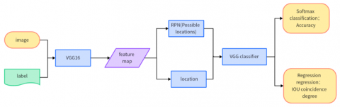
Figure 8. Workflow of the VGG16 backbone model
The training process is as follows:
(1) Feature Map Extraction: Labeled original images go through the Conv+ReLU+Pooling layers of ResNet50, extracting the Input image's Feature maps. These Feature maps are used for subsequent RPN layers and layers beyond.
(2) RPN: Primarily utilizes a sliding window to connect to the Feature map output by the last convolutional layer of the CNN network, taking the feature map as the input to the output layer. After generating a set of Anchor boxes, a Softmax determines if these Anchors are foreground or background. Signal changes are considered foreground, and the rest as non-foreground, akin to a binary classification problem; during the R-CNN process, the generated proposals undergo IOU evaluation, with those over 0.7 considered foreground, identifying possible lesion locations. Additionally, another branch of the network regresses these Anchor boxes for proposal refinement, aiming for precision.
(3) ROI Pooling: Receives the Feature map from the last layer of the CNN ResNet50 and the refined proposals generated by RPN. After ROI Pooling, a fixed-size proposal feature map is obtained, which is then fed into the subsequent network for target recognition and localization operations using full connections.
(4) Model Tail: Consists of a Softmax classifier and a bounding box regressor (b-box regressor). The fixed-size Feature map formed by the ROI Pooling layer undergoes a full connection operation (compared to R-CNN, SPP Net in classification). Faster R-CNN has two network output layers, integrating the separately operated b-box regression into a unified network in a formal sense and simultaneously constructing a loss function that optimizes both output layers. The network architecture includes four loss functions (rpn_cls_loss, rpn_box_loss, rcnn_cls_loss, rcnn_box_loss), with RPN and Fast R-CNN each having their own classifiers and regressors.
5.4.3 VGG16 faster R-CNN training process
The Faster R-CNN network based on VGG16, compared to the ResNet network, has slight differences in feature extraction by the convolutional layers. The subsequent processes, shown in Figure 8, including the RPN layer, Pooling layer, and full connections for classification and target localization, are essentially the same:
(1) Images are input into a VGG-16 network for feature extraction; resulting in a set of Feature maps, similar to ResNet50, with Feature map=38*50;
(2) Potential lesion locations are determined through the RPN network;
(3) These location information is located on the Feature map through the ROI Pooling layer;
(4) Finally, the region information obtained through the VGG-16 classifier and IOU are evaluated for overlap degree, integrated into a function and backpropagated, completing a training round.
In order to verify the efficiency of different deep learning models, this paper simultaneously compared the differences in detection methods and image detection speed of RCNN, Fast-RCNN, and Fast-RCNN, as shown in Table 6.
Table 6. Comparison of three network detection methods and their speeds
|
Project |
R-CNN |
Fast-RCNN |
Faster-RCNN |
|
Extract candidate box |
Selective Search |
Selective Search |
RPN network |
|
Feature Extraction |
Convolutional Neural Network (CNN) |
Convolutional Neural Network+ ROI Pooling |
|
|
Feature classification |
SVM |
||
|
Image detection time (proposals collected) |
50S |
2S |
0.2S |
|
Acceleration |
1X |
25X |
250X |
This study utilizes Faster R-CNN from deep learning and CNNs such as VGG-16 and Resnet50 to identify and predict areas of SCI in MRI images. After model validation with a validation set and optimization through iterative updates of the best parameters, the trained models were tested with a test set to determine their predictive accuracy. In clinical practice, evaluating the prediction effectiveness of a disease solely based on recall or accuracy rates is not meaningful. Therefore, in terms of model efficiency evaluation, we mainly chose mAP for assessment. During the prediction phase, 500 images were selected as a test set to verify and compare the effectiveness of network models based on VGG-16 and Resnet50.
In this experiment's network data, the overall mAP results obtained after processing the prediction set through the two models (VGG-16 and Resnet50) were 72.3% and 88.6%, respectively. Another metric for measuring model computational efficiency is the detection speed. In terms of detection speed, when the test set images were processed using VGG-16 and Resnet50 models, the testing speeds were 0.24s/image and 0.22s/image, respectively. A comparison of the overall network effects of the two models is shown in Table 7, with main evaluation metrics including detection mAP and overall detection time.
After processing 500 images from the test set through the trained network models, the models sequentially predict and output visualization images, as shown in Figure 9, which includes some visualization results of edematous and lumbar disc herniation. Each image contains bounding boxes around the target area, along with the corresponding classification name and predicted probability value. These appropriately sized bounding boxes and predicted probabilities directly reflect the credibility of the disease. In Figure 9 below, representing a subset of the prediction set results, the credibility of SCI signals and the corresponding bounding boxes can be clearly seen, showing the location of the SCI signals within the bounding boxes and their corresponding credibility. This presentation of visualization results allows for direct observation of the predictive effectiveness of the images.
Table 7. Comparison of recognition results between different network models
|
Algorithm |
Network Model |
mAP (%) |
Detection Speed (sec/image) |
|
Faster R-CNN |
Resnet50 |
88.6 |
0.22 |
|
Faster R-CNN |
VGG-16 |
72.3 |
0.24 |
Figure 9. Example of visualization results
This paper presents a method based on deep learning for SCI analysis, aimed at accurately detecting, identifying, and marking the presence of SCI within MRI images, including their location, size, and prediction probability. This method represents a shift from qualitative to quantitative analysis of SCI, effectively narrowing the diagnostic gap due to varying levels of clinical experience and improving diagnostic accuracy, reducing workload, and overcoming the limitations, randomness, and uncontrollability of SCI diagnosis and treatment. This paper demonstrated that the application of the Faster R-CNN algorithm with neural network models based on VGG-16 and ResNet50 can recognize and detect common diseases such as spinal disc herniation and changes in spinal cord signals. Using standardized datasets, selecting appropriate models, and evaluation criteria can lead to satisfactory experimental results. However, the network architecture model based on ResNet50 outperforms the one based on VGG-16 in terms of predictive effect and detection speed, indirectly proving that deeper network structures help improve prediction effects. It also confirms the theoretical effectiveness of the big data + artificial intelligence model.
The innovative content of this article is as follows: (1) Using the current hot topic of deep learning technology in artificial intelligence - Faster R-CNN, to explore whether it can recognize and detect common cervical spine diseases in magnetic resonance imaging, in order to verify the feasibility and effectiveness of deep learning technology for diseases in this field. (2) This paper adopts the method of object recognition detection in deep learning to locate and predict common cervical spine diseases, and compares experiments with different network structures. It is found that the deeper the neural network, the better the training effect. (3) The successful recognition and detection of common diseases in the cervical spine using deep learning technology has laid the theoretical foundation for clinical application of cervical spine disease MRI+deep learning mode. Of course, there are still certain challenges from theoretical foundations to model integration and practical clinical workflows, such as accuracy, transparency, and interpretability, as well as concerns about data privacy and security. In terms of accuracy, the training data of deep learning models for spinal cord injury detection is relatively scarce due to the involvement of privacy, and the accuracy needs to be improved. During the training process of the large model, it is necessary to strengthen data validation, increase uncertainty indicators, optimize medical accuracy, and self improve through error correction algorithms and other methods. In terms of transparency and interpretability, it is not yet clear how the model generates answers (black box questions) from input queries and data structures, nor is it clear which parts of the training dataset are used in the result response. To solve this problem, it is necessary to reference the data section that contributes to the answer in the model output, and conduct in-depth research and development of interpretable AI. The application of large models in the medical field faces multiple technical challenges and limitations, such as insufficient knowledge, limited interpretability and accuracy, coherence intersections, and model hallucinations. Overcoming these issues requires interdisciplinary collaboration, strengthening data management and protection, researching interpretable AI methods, and continuously improving the performance and security of models to ensure their reliability and effectiveness in medical practice.
Certainly, this paper has some limitations, such as in data collection, where there may be issues like insufficient structural quality of data, small data volume, incomplete indication data, and difficulty in sharing. The completeness and accuracy of data can affect the performance of the neural network model; the deep learning model is still not perfect, and there is room for improvement in detection accuracy. Future research directions should continue to investigate the causes of misdiagnosis and missed diagnosis, consider designing a correction module, and use correction algorithms to correct the automatic detection results of the trained spinal cord analysis neural network. After image detection is complete, a comparison of the signal differences recognized by T2WI and T2 fat suppression should be conducted, followed by a comparison at the same level and dimension. After the comparison, match analysis weight to correct instances where some interferences are mistakenly identified as SCI.
This research was supported by Zhejiang Provincial Basic Public Welfare Research Project (Grant No.: LTGY23H170005) and Zhejiang Provincial Health Science and Technology Plan (Project No.: 2024KY644).
[1] Patek, M., Stewart, M. (2002). Spinal cord injur. Anaesthesia & Intensive Care Medicine, 24(7): 406-411. https://doi.org/10.1016/j.mpaic.2023.04.006
[2] Hersh, A.M., Weber-Levine, C., Jiang, K., Theodore, N. (2023). Spinal cord injury: Emerging technologies. Neurosurgery Clinics, 35(2): 243-251. https://doi.org/10.1016/j.nec.2023.10.001
[3] Thorogood, N.P., Waheed, Z., Chernesky, J., Burkhart, I., Smith, J., Sweeney, S., Noonan, V.K. (2023). Spinal cord injury community personal opinions and perspectives on spinal cord stimulation. Topics in Spinal Cord Injury Rehabilitation, 29(2): 1-11. https://doi.org/10.46292/sci22-00057
[4] Wang, H., Xiang, Q., Li, C., Zhou, Y. (2013). Epidemiology of traumatic cervical spinal fractures and risk factors for traumatic cervical spinal cord injury in China. Clinical Spine Surgery, 26(8): E306-E313. https://doi.org/10.1097/BSD.0b013e3182886db9
[5] Hamid, R., Averbeck, M.A., Chiang, H., Garcia, A., Al Mousa, R.T., Oh, S.J., Del Popolo, G. (2018). Epidemiology and pathophysiology of neurogenic bladder after spinal cord injury. World Journal of Urology, 36: 1517-1527. https://doi.org/10.1007/s00345-018-2301-z
[6] Vadassery, S.J., Seneviratna, A., Ho, E.W., Dalan, R. (2023). Polyuria after spinal cord injury. Singapore Medical Journal, 2023, https://doi.org/10.4103/singaporemedj.SMJ-2020-532
[7] Gupta, S., McColl, M.A., Smith, K., McColl, A. (2023). Prescribing patterns for treating common complications of spinal cord injury. The Journal of Spinal Cord Medicine, 46(2): 237-245. https://doi.org/10.1080/10790268.2021.1920786
[8] Bluvshtein, V., Catz, A., Mahamid, A., Elkayam, K., Michaeli, D., Kfir, A., Aidinoff, E. (2023). Venous thromboembolism and anticoagulation in spinal cord lesion rehabilitation inpatients: A 10-year retrospective study. NeuroRehabilitation, 53(1): 143-153. https://doi.org/10.3233/NRE-230063
[9] Vecin, N.M., Gater, D.R. (2022). Pressure injuries and management after spinal cord injury. Journal of Personalized Medicine, 12(7): 1130. https://doi.org/10.3390/jpm12071130
[10] Matsumoto, Y., Hayashi, T., Fujiwara, Y., Kubota, K., Masuda, M., Kawano, O., Maeda, T. (2023). Correlation between respiratory dysfunction and dysphagia in individuals with acute traumatic cervical spinal cord injury. Spine Surgery and Related Research, 7(4): 327-332. https://doi.org/10.22603/ssrr.2022-0180
[11] Gurung, S., Jenkins, H.T., Chaudhury, H., Ben Mortenson, W. (2023). Modifiable sociostructural and environmental factors that impact the health and quality of life of people with spinal cord injury: A scoping review. Topics in Spinal Cord Injury Rehabilitation, 29(1): 42-53. https://doi.org/10.46292/sci21-00056
[12] Pfyffer, D., Freund, P. (2021). Spinal cord pathology revealed by MRI in traumatic spinal cord injury. Current Opinion in Neurology, 34(6): 789-795. https://doi.org/10.1097/WCO.0000000000000998
[13] Anantharajan, S., Gunasekaran, S., Subramanian, T., Venkatesh, R. (2024). MRI brain tumor detection using deep learning and machine learning approaches. Measurement: Sensors, 31: 101026. https://doi.org/10.1016/j.measen.2024.101026
[14] Bousis, D., Verras, G.I., Bouchagier, K., Antzoulas, A., Panagiotopoulos, I., Katinioti, A., Mulita, F. (2023). The role of deep learning in diagnosing colorectal cancer. Gastroenterology Review/Przegląd Gastroenterologiczny, 18(3): 266-273. https://doi.org/10.5114/pg.2023.129494
[15] Lundervold, A.S., Lundervold, A. (2019). An overview of deep learning in medical imaging focusing on MRI. Zeitschrift für Medizinische Physik, 29(2): 102-127. https://doi.org/10.1016/j.zemedi.2018.11.002
[16] de Paiva, J.L., Sabino, J.V., Pereira, F.V., Okuda, P.A., de Lima Villarinho, L., de Souza Queiroz, L., Reis, F. (2023). The role of MRI in the diagnosis of spinal cord tumors. In Seminars in Ultrasound, CT and MRI. WB Saunders, 44(5): 436-451. https://doi.org/10.1053/j.sult.2023.03.012
[17] Zhang, Z., Zhu, Z., Liu, D., Wang, X., Liu, X., Mi, Z., Fan, H. (2024). Machine learning and experiments revealed a novel pyroptosis-based classification linked to diagnosis and immune landscape in spinal cord injury. Heliyon, 10(3): e24974. https://doi.org/10.1016/j.heliyon.2024.e24974
[18] Kim, Y., Lim, M., Kim, S.Y., Kim, T.U., Lee, S.J., Bok, S.K., Hyun, J.K. (2024). Integrated machine learning approach for the early prediction of pressure ulcers in spinal cord injury patients. Journal of Clinical Medicine, 13(4): 990. https://doi.org/10.3390/jcm13040990
[19] Jazayeri, S.B., Maroufi, S.F., Akbarinejad, S., Ghodsi, Z., Rahimi-Movaghar, V. (2024). Development of a regional-based predictive model of incidence of traumatic spinal cord injury using machine learning algorithms. World Neurosurgery: X, 23: 100280. https://doi.org/10.1016/j.wnsx.2024.100280
[20] Ke, G., Liao, H., Chen, W. (2023). Clinical manifestations and magnetic resonance imaging features of spinal cord infarction. Journal of Neuroradiology. https://doi.org/10.1016/j.neurad.2023.10.003
[21] Szaro, P., Geijer, M., Ciszek, B., McGrath, A. (2022). Magnetic resonance imaging of the brachial plexus. Part 2: Traumatic injuries. European Journal of Radiology Open, 9: 100397. https://doi.org/10.1016/j.ejro.2022.100397
[22] Chang, C., Zhu, J., Li, H., Yang, Q. (2022). Enhanced magnetic resonance imaging manifestations of paediatric intervertebral disc calcification combined with ossification of the posterior longitudinal ligament: Case report and literature review. BMC pediatrics, 22(1): 400. https://doi.org/10.1186/s12887-022-03461-5
[23] Garcea, F., Serra, A., Lamberti, F., Morra, L. (2023). Data augmentation for medical imaging: A systematic literature review. Computers in Biology and Medicine, 152: 106391. https://doi.org/10.1016/j.compbiomed.2022.106391
[24] Umer, M., Ashraf, I., Ullah, S., Mehmood, A., Choi, G. S. (2022). COVINet: A convolutional neural network approach for predicting COVID-19 from chest X-ray images. Journal of Ambient Intelligence and Humanized Computing, 13(1): 535-547. https://doi.org/10.1007/s12652-021-02917-3
[25] Sowrirajan, S.R., Balasubramanian, S., Raj, R.S.P. (2022). MRI brain tumor classification using a hybrid VGG16-NADE model. Brazilian Archives of Biology and Technology, 66: e23220071. https://doi.org/10.1590/1678-4324-2023220071
[26] Sharma, S., Guleria, K., Tiwari, S., Kumar, S. (2022). A deep learning based convolutional neural network model with VGG16 feature extractor for the detection of Alzheimer Disease using MRI scans. Measurement: Sensors, 24: 100506. https://doi.org/10.1016/j.measen.2022.100506
[27] Hassan, S.M., Maji, A.K. (2024). Pest Identification based on fusion of Self-Attention with ResNet. IEEE Access, 12: 6036-6050. https://doi.org/10.1109/ACCESS.2024.3351003
[28] El Ariss, O., Hu, K. (2022). ResNet-based Parkinson's disease classification. IEEE Transactions on Artificial Intelligence, 4(5): 1258-1268. https://doi.org/10.1109/TAI.2022.3193651
[29] Pan, H., Zhang, H., Lei, X., Xin, F., Wang, Z. (2022). Hybrid dilated faster RCNN for object detection. Journal of Intelligent & Fuzzy Systems, 43(1): 1229-1239. https://doi.org/10.3233/jifs-212740