Binghua Nie![]() | Bin Ma*
| Bin Ma*![]()
© 2024 The authors. This article is published by IIETA and is licensed under the CC BY 4.0 license (http://creativecommons.org/licenses/by/4.0/).
OPEN ACCESS
The prevalence of cheating in first-person shooter (FPS) games poses a formidable challenge, undermining user experience and the integrity of competitive play. In response to this issue, a visual-based anti-cheating detection network, termed VADNet, has been developed, harnessing the capabilities of deep learning and computer vision techniques. VADNet incorporates a focus module designed to segment high-resolution images, alongside a Feature Pyramid Network (FPN) for the fusion of multi-scale features, culminating in a classifier module tasked with the quantification of cheating behaviors. Rigorous experimentation on a dataset derived from a real online FPS game substantiates VADNet's efficacy in identifying players who resort to cheating, as evidenced by high precision, recall, and F1 scores. This investigation advances the field of anti-cheating mechanisms for FPS games, offering a robust and reliable system to preserve the fairness and integrity of online gaming environments.
cheat detection, first-person shooter (FPS) games, visual algorithm
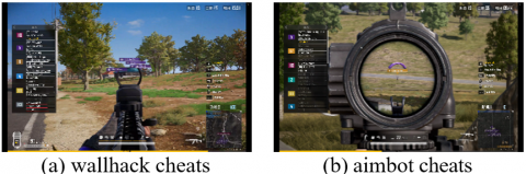
FPS games are a highly competitive genre with demanding requirements for reaction speed, and they have become one of the mainstream categories in the current gaming market [1-4]. Simultaneously, the issue of cheating has emerged as a major challenge in the FPS gaming industry, impacting the gaming ecosystem and players’ overall gaming experience. Recent data indicates that in the first half of 2023, there were a cumulative 3.2 billion detections of cheating in mobile games, marking a 40% year-over-year increase. Among these, the most prevalent type of cheat used in FPS games is wallhack, accounting for 58.33% of the total, while aimbot, despite only representing 8.33%, has the most significant impact on user experience, as shown in Figure 1. Therefore, detecting and identifying cheating has become an urgent and imperative problem that needs immediate resolution in the FPS gaming industry.
The genre of shooting games, unlike card games and others that do not require a focus on real-time client-side calculations, exhibits significant differences. To ensure a smooth gaming experience in shooting games, many gameplay calculation logics need to be executed locally on the client-side [5]. This makes it impractical to adopt server-side validation methods, laying the groundwork for cheating through hacks. Utilizing cross-process hacks with elevated privileges enables the extraction of crucial game logic data, allowing for features such as wallhacks through external rendering processes. In this scenario, the game logic executes without any anomalies, and the game remains unaware of the detailed information related to the hacking process. Alternatively, modifying shader data can influence the GPU rendering process, enabling features like perspective rendering, character coloring, and removing grass and trees. These challenging hacks are difficult for conventional anti-cheat measures to handle and detect. Therefore, this study adopted a visual approach using deep learning to discern and counteract these issues.
Figure 1. Common cheating methods
This paper proposes a deep learning and visual analysis-based FPS anti-cheat model, aimed at detecting the use of cheats by analyzing player behavior in game videos. The logical patterns of players’ in-game actions are examined, and visual recognition techniques are employed, allowing the model to effectively determine the presence of cheating behavior, irrespective of the cheat type involved. To achieve the anti-cheat objectives, three key challenges must be addressed:
Challenge 1: Recognizing Visual Disparities
The use of deep learning for visual detection of cheating has been identified as a promising approach [6-8], attributed to significant visual differences between normal players and cheaters. This method, which does not require additional privacy information and relies solely on reliable image data [9], faces the challenge of accurately identifying these visual differences.
Challenge 2: Quantifying Cheating Behavior
The often subtle and difficult-to-detect behavioral differences manifested by cheating behavior necessitate real-time capabilities in cheating detection systems [10, 11]. Furthermore, the quantification of appropriate cheating detection indicators and the design of a reasonable detection system are demanded, ensuring the system's ability to accurately and rapidly respond to various situations [12, 13].
Challenge 3: Enhancing Credibility
It is crucial for anti-cheat system design to ensure accurate cheating detection without falsely identifying legitimate players as cheaters. The critical challenge lies in improving target detection and cheat classification accuracy, reducing false-positive rates to avoid negatively impacting legitimate players, and enhancing the overall credibility of the cheat detection system [14, 15].
Contributions are as follows: (1) A visual-based FPS game anti-cheat network has been developed, achieving comprehensive cheat detection through supervised learning on datasets of normal gaming and cheating scenarios. (2) By detecting and categorizing player behavior, a set of key performance indicators has been introduced. Monitoring the relative relationships between actions such as aiming frequency, effective aiming duration, and kill count enables the more accurate capture of differences between cheating players and regular players. (3) Extensive experiments and analyses conducted on a real online FPS game dataset have demonstrated the network's effectiveness and potential in detecting players using cheats.
2.1 Traditional methods
Park and Lee [16] categorized methods for detecting game cheats into three types: player client detection, game network communication detection, and game remote server detection. In the case of Player Unknown’s Battlegrounds (PUBG), the Battle Eye system employed by the game continuously collects information on all processes in the user’s memory. It randomly extracts files from the player’s computer for analysis. However, this inevitably raises a series of privacy concerns. Yu et al. [17] investigated the situation where players’ clients send data packet commands to the server. They monitored different amounts of traffic during various time periods to identify changes in traffic when cheats were used compared to normal gameplay. However, cunning cheaters often employ techniques such as traffic obfuscation, encryption, and confusion to bypass detection. Some games, like "Fantasy Westward Journey" and "Dungeon & Fighter," intermittently present image captchas or numeric quizzes during gameplay to determine if users are present [18]. However, the effectiveness of these anti-cheat methods, based on pop-up event detection, has gradually diminished due to advancements in facial recognition and image processing technologies.
2.2 Deep learning methods
Traditional cheating detection systems often struggle to be effective against new vulnerabilities or sophisticated cheaters. With the advancement of artificial intelligence (AI) technology, methods based on image processing and AI have been widely explored in the field of cheating detection by
many researchers. Galli et al. [19]. developed AI agents resembling human players by analyzing human player behavior using various methods. However, this approach has low accuracy and requires human involvement, resulting in inefficiency. Spijkerman and Marie Ehlers [20] applied Support Vector Machines (SVMs), decision trees, and Naive Bayes machine learning models to analyze players’ mouse and keyboard operations. By integrating learning features into SVM models, they achieved superior cheating detection results. However, relying solely on SVMs for cheating detection may overlook crucial information such as players’ aiming frequency, hit rates, and pre-aim positions [21]. Some researchers have used Recurrent Neural Networks (RNNs) to detect cheating. However, RNNs’ sequential computation process leads to high computational complexity during training and inference. This limitation restricts the scalability and accuracy of RNNs when dealing with long sequences or large-scale tasks [22-24].
In comparison to traditional image processing methods, deep learning can automatically learn and extract features from images without relying on manually designed feature extractors [25-27]. Through the combination and training of multiple layers of neural networks, deep learning excels at extracting advanced features from complex images. Deep learning has achieved significant success in areas such as image recognition, object detection, image enhancement, and image reconstruction. In the context of game cheating detection, deep learning’s capabilities are evident, as exemplified by the automatic recognition of cheating behavior patterns, such as "aimbot," in players of games like PUBG. These models leverage extensive datasets of player behavior features to accurately identify key cheating indicators, providing essential auxiliary criteria for the detector’s judgment [28-30].
2.3 Preliminary
This section provides an overview of object detection and the important definitions used in the employed models. Additionally, a concise summary of commonly used symbols is given in Table 1.
Table 1. Notations and definitions
|
Notations |
Definitions |
|
W |
Convolutional layer parameter matrix |
|
ω |
Width of the image or bounding box |
|
ℎ |
Height of the image or bounding box |
|
c |
Number of channels |
|
BN |
Batch normalization |
|
IoU |
Intersection over Union |
|
Ttg |
Effective targeting time |
|
Ntg |
Effective targeting count |
1. Intersection over Union (IoU)
Defined as the intersection area of two rectangular boxes divided by their union area, expressed by the following formula:
$I o U=\frac{|A \cap B|}{|A \cup B|}$ (1)
2. Batch Normalization (BN)
BN normalizes the variance and mean of features across examples within each small batch, aiming to prevent issues like gradients vanishing or exploding.
3. Max pooling
Pooling layers down sample each input feature map by utilizing a 2×2 max-pooling window with a stride of 2, achieving a reduction in the spatial dimensions of the input data.
4. Effective targeting
The duration during which aiming is detected, and a person is recognized in the viewfinder is considered the effective targeting time in object detection.
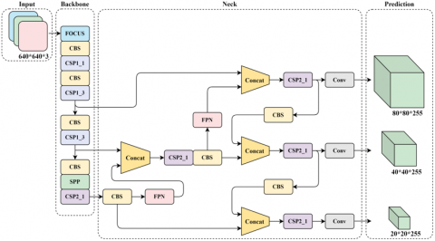
This section introduces the proposed vision-based anti-cheating detection model, as shown in Figure 2, which consists of four key modules: the data preprocessing module, backbone module, neck module, and head module. Images from the dataset are first concatenated and padded through the data preprocessing module. Subsequently, the backbone module splits and applies convolutional operations to extract features from the images. Pooling operations are then used to merge the feature vectors. The neck module serves as a connecting module to further optimize and fuse features to adapt to the downstream tasks. Finally, the head module calculates the loss function and classifies the indicators of cheating through the classifier module for output.
3.1 Data preprocessing module
The data preprocessing module primarily involves scaling the input images to the network's input size and normalizing them. During the model training phase, this module employs Mosaic data augmentation operations to concatenate multiple images into a new complete photo for data input, using random scaling, random cropping, and random arrangement. This approach not only enhances the training speed of the model but also reduces its memory requirements.
The module utilizes adaptive anchor box calculation, with the formula as follows:
$\begin{aligned} & r=\frac{w}{h} \\ & N_m=\left\{\begin{array}{l}N_m+1, \text { if } \min \left(\frac{w_b}{h_b}\right)<\max \left(\frac{w_a}{h_a}\right) \\ N_m, \text { otherwise }\end{array}\right. \\ & R=\frac{N_m}{N_t} \\ & \end{aligned}$ (2)
r represents the aspect ratio. Initially, utilizing n bounding boxes and 9 anchor boxes, the aspect ratio r is calculated. If the maximum aspect ratio (r) of the anchor boxes is greater than the minimum aspect ratio (r) of the bounding boxes, it is considered a successful match. If the probability of a successful match is less than 98%, a genetic algorithm and k-means are employed to recalculate the anchors, and the anchor box with the highest success rate is saved.
Adaptive image scaling techniques have been incorporated, and the formula is as follows:
$\alpha=\min \left(\frac{w_0}{w_1}, \frac{h_0}{h_1}\right)$ (3)
$\begin{gathered}w_1=\alpha \cdot w_1=\alpha \cdot h \\ d w=w_1-w_0 \\ d h=h_1-h_0\end{gathered}$ (4)
Figure 2. Illustration of the proposed VADNet anti-cheating detection model
Calculate the minimum scaling factor α between the target image and the original image. Then, multiply the height and width of the target image by α to compute the size of the scaled image. Finally, adaptively calculate the padding values for convolution and pooling in the model based on the scaled image size, accounting for potential black borders.
3.2 Backbone module
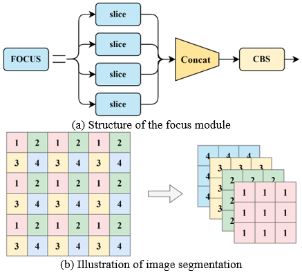
The backbone module introduces the focus module to segment the image, splitting the high-resolution image (feature map) into multiple low-resolution images or feature maps.
The input $x \in \mathbb{R}^{b \times c \times w \times h}$ undergoes the focus layer to obtain $\hat{x} \in \mathbb{R}^{b \times 4 c \times \frac{w}{2} \times \frac{h}{2}}$, where the channel count is quadrupled compared to the original RGB three-channel mode. The final result $\hat{x}$ is a feature map with twice the down-sampling without losing information, as depicted in Figure 3.
Figure 3. Process of the focus module
After this image is subjected to another convolution operation, it results in $y \in \mathbb{R}^{b \times c' \times \times \frac{w}{2} \times \frac{h}{2}}$, as depicted in Figure 3. The formula for this process is as follows:
$y=f\left(\sum_{c=1}^c \hat{x}_c * W_{\left(c, c^{\prime}\right)}+b_{\left(c^{\prime}\right)}\right)$ (5)
The input feature map comprises c input channels $\left(\hat{x}_1: \hat{x}_2: \hat{x}_3: \ldots: \hat{x}_c\right)$ and c' output channels $\left(y_1: y_2: y_3: \ldots: y_{c^{\prime}}\right)$. The weight parameters of this CONV layer have the shape [filter_height, filter_width, in_channels, out_channels], denoted by $W_{\left(c, c^{\prime}\right)} \in \mathbb{R}^{r \times r \times c \times c^{\prime}}$. Here, f represents the activation function, and $b_{c^{\prime}}$ is the bias term for the output feature maps of the same size.
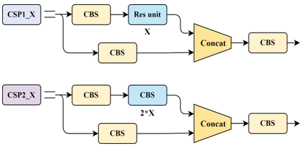
The output y undergoes several CSP1_X and CSP2_X layers. The structure of CSP1_X is illustrated in Figure 4, and the corresponding formula is as follows:
$\begin{gathered}y_1=f\left(\sum_{c=1}^c y^* W_{\left(c, c^{\prime}\right)}+b_{c^{\prime}}\right) \\ \hat{y}_2=\operatorname{CBL}(y)\end{gathered}$ (6)
$\begin{gathered}\hat{y}_2^{\prime}=\underbrace{\operatorname{Res}\left(\hat{y}_2\right) \mid\left(\operatorname{Res}\left(\hat{y}_2\right)\|\ldots\| \operatorname{Res}\left(\hat{y}_2\right)\right)}_X \\ y_2=f\left(\sum_{c=1}^c \hat{y}_2^{\prime} * W_{\left(c, c^{\prime}\right)}+b_{c^{\prime}}\right)\end{gathered}$
Figure 4. Schematic diagram of submodule construction
The Convolutional Block Layer (CBL) sums over all input channels, multiplying each channel by the corresponding weights and adding biases. The formula for feature extraction using the Res (Residual) method is as follows:
$\begin{gathered}\operatorname{CBL}(y)=\operatorname{ReLU}\left(\operatorname{BN}\left(\sum_{c=1}^c y^* W_{\left(c, c^{\prime}\right)}+b_{c^{\prime}}\right)\right) \\ \operatorname{Res}(y)=y+\operatorname{CBL}(\operatorname{CBL}(y))\end{gathered}$ (7)
The CBL structure consists of three network layers: Convolution (Conv), Batch Normalization, and Leaky ReLU. In CSP1_X, we go through several CBL structures and concatenate residuals to obtain the final output $\hat{y}$. CSP2_X is similar to CSP1_X, but the Res part is replaced with 2X CBL structures. The formulas are as follows:
$\begin{gathered}y_1=f\left(\sum_{c=1}^c y^* W_{\left(c, c^{\prime}\right)}+b_{c^{\prime}}\right) \\ \hat{y}_2=\operatorname{CBL}(y) \\ \hat{y}_2^{\prime}=\underbrace{\operatorname{CBL}\left(\hat{y}_2\right) \mid\left(\operatorname{CBL}\left(\hat{y}_2\right)|\ldots| \operatorname{CBL}\left(\hat{y}_2\right)\right)}_{2 X}\end{gathered}$ (8)
$\begin{gathered}y_2=f\left(\sum_{c=1}^c \hat{y}_2^{\prime} * W_{\left(c, c^{\prime}\right)}+b_{c^{\prime}}\right) \\ \hat{y}=\operatorname{ReLU}\left(\operatorname{BN}\left(y_1 \| y_2\right)\right)\end{gathered}$ (9)
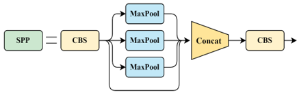
Figure 5. SPP module illustration
As shown in Figure 5, SPP performs max pooling on each feature map using three different sizes of pooling kernels to obtain predetermined feature map sizes. Finally, all feature maps are flattened into feature vectors and fused.
3.3 Neck module
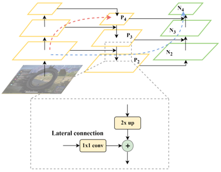
The Neck network is a crucial component in object detection algorithms, responsible for further optimizing and fusing features extracted by the backbone network to better adapt to the requirements of object detection tasks, as illustrated in Figure 6. The FPN is a top-down process that transfers and fuses high-level feature information through upsampling to obtain feature maps for prediction, allowing the network to perform object detection at multiple scales. In the bottom-up stage, images are input into the backbone network, and features with different scales of information are extracted using CSP1_X, CSP2_X, and Conv. In the top-down stage, the feature maps obtained at higher levels are transmitted to the lower levels through upsampling, enriching the semantic information in the lower-level feature maps. Finally, in the Lateral Connection process, the features obtained by upsampling the higher-level feature maps are fused with the lower-level feature maps, and the fusion can be a simple addition or a 1×1 convolution. After fusion, a fused feature map is generated at each scale, forming a feature pyramid. This feature pyramid contains semantic information at different scales, enabling the model to detect objects at different scales. Although FPN has already integrated shallow features once, it still cannot achieve satisfactory segmentation results. Therefore, PAN is introduced, enhancing the network's perception of multi-scale information through a mechanism that fuses features along both lateral and contextual paths.
Figure 6. FPN-PAN structure
As shown in Figure 6, it involves downsampling N2 (N2 and P2 are the same feature map, so N2 already contains a considerable amount of low-level features). The downsampled feature map is then fused with P3 to obtain N3. Therefore, N3 contains more low-level features than P3, and this pattern continues for N4, N5, and so forth.
3.4 Head module
The model has three main loss functions: Classification Loss (cls_loss), responsible for determining whether the classification of anchor boxes matches the annotations; Localization Loss (box_loss), which measures the error between predicted boxes and annotated boxes (GIoU); and Confidence Loss (obj_loss), which calculates the network's confidence. Binary cross-entropy loss functions are employed for both classification and localization losses, as represented by the following formulas:
$C=-\frac{1}{n} \sum[y \ln a+(1-y) \ln (1-a)]$ (10)
where, x represents the sample, y represents the label, a represents the predicted output, and n represents the total number of samples. The confidence loss calculation adopts the CIOU_Loss as the bounding box loss function, and the formula is as follows:
$\mathrm{CIOU}_{\text {Lass }}=\mathrm{IOU}-\frac{\rho^2\left(b, b^{g t}\right)}{c^2}-\alpha v$ (11)
where, IOU is the intersection over union between the predicted box and the ground truth box. $\rho^2\left(b, b^{g t}\right)$ represents the Euclidean| distance between the center points of the predicted box and the ground truth box. c denotes the diagonal distance of the minimum closed region that can simultaneously contain the predicted box and the ground truth box.
$\begin{gathered}\alpha=\frac{v}{1-I O U+v} \\ v=\frac{4}{\pi^2}\left(\arctan \left(\frac{w^{g t}}{h^{g t}}\right)-\arctan \left(\frac{w}{h}\right)\right)^2\end{gathered}$ (12)
where, wgt and hgt are the width and height of the ground truth bounding box, and w and h are the width and height of the predicted bounding box. Additionally, the output end of the Head module adopts sigmoid as the activation function, addressing the issue of slow weight updates in the loss function.
3.5 Classifier module
The differentiation in the ratios of duration, frequency, and kill effectiveness in aiming between normal players and those suspected of cheating is analyzed. Data standards are quantified to ascertain the usage of cheats by a player. The calculation of the duration of effective aiming is conducted by recognizing the period during which the player aims and maintains the target within sight. The duration ratio is subsequently calculated by dividing the duration of effective aiming by the total operational time of the aiming mechanism. The formula is delineated as follows:
$\beta_T=\frac{T_t g}{T_A}$ (13)
where, TA represents the total time with the sight open, calculated by the continuous duration of the aiming action detected through target recognition. The ratio of effective aiming instances is the number of times effective aiming occurs divided by the total number of times the sight is open.
$\beta_N=\frac{N_t g}{N_A}$ (14)
The ratio of scoped kills is the quotient of the number of kills and the number of times the sight is opened.
$\beta_K=\frac{N_K}{N_A}$ (15)
In the process of normal player behavior, there is ineffective scoping, i.e., situations where there is no one in sight. However, for cheating players, the ratios of effective scoping occurrences $\left(\beta_N\right)$ and effective scoping duration $\left(\beta_T\right)$ are significantly higher than those of normal players, and the scoped kill ratio $\left(\beta_K\right)$ is also higher. By quantifying and statistically analyzing the differences in these three indicators between normal players and cheaters, we can classify whether cheating is involved.
4.1 Datasets
Our dataset consists of videos collected from online FPS games provided by a network company, ensuring privacy protection. Frames from the videos were processed and cut into numerous images, and the self-made dataset was created through preprocessing and labeling, resulting in training, testing, and validation sets. The basic statistics of the dataset are summarized in Table 2.
Table 2. Basic statistics of the dataset
|
Dataset |
Size |
#Sample |
|
Train |
640×640 |
2115 |
|
Valid |
640×640 |
200 |
|
Test |
640×640 |
100 |
4.2 Experiment settings
The experiment runs on a device equipped with an NVIDIA Tesla T4 16GB GPU. In this experiment, the model undergoes training for 100 epochs with a batch size of 16, and the images are resized to 640×640 pixels. Multi-scale training is applied, treating the dataset as a single category. The SGD optimizer and synchronized batch normalization are utilized. A quarter-sized data loader is employed, and a cosine learning rate scheduler is used. Label smoothing is set to 0.0, and early stopping waits for 100 epochs.
4.3 Evaluation metrics
Three common metrics are employed for evaluation, including precision, recall, and F1 score. Additionally, a confusion matrix is plotted to illustrate the correct recognition scenarios (see Table 3).
Table 3. Different recognition scenarios
|
Total Population (P+N) |
Positive (PP) |
Negative (NN) |
|
Positive (P) |
True Positive (TP) |
False Negative (FN) |
|
Negative (N) |
False Positive (FP) |
True Negative (TN) |
1. Precision
$P=\frac{T P}{(T P+F P)}$ (16)
Therefore, P (Precision) refers to the proportion of correctly predicted positive samples (TP) among all samples predicted as positive TP+FP. An increase in P indicates that the model's judgments of "predicted positive" are more reliable, meaning that the model more accurately identifies positive instances.
2. Recall
$R=\frac{T P}{(T P+F N)}$ (17)
Recall, starting from true positive labels, calculates the proportion of correctly predicted positive samples (TP) among all true positive samples (TP+FN). A higher recall is desirable as it indicates that the model makes fewer false negatives and has a lower probability of missing actual positive instances.
3. F1-Score
$F_\beta=\frac{\left(1+\beta^2\right) \times(P \times R)}{\beta^2 \times P+R}$ (18)
When β=1, the term is referred to as the F1-Score, which assigns equal importance to Recall and Precision, amalgamating these two metrics into a singular measure.
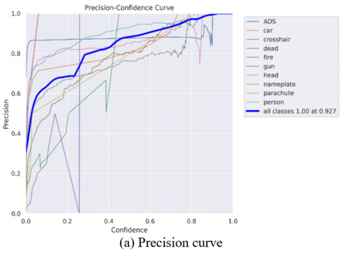
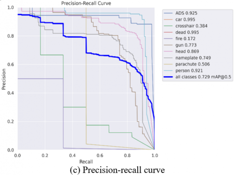
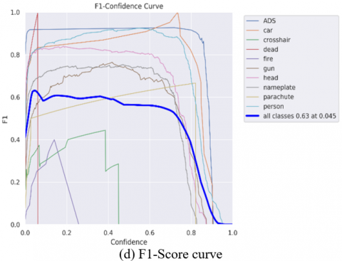
Figure 7. Evaluation metrics on the dataset
4.4 Experiment result
As shown in Figure 7, it can be observed that P is 1.00, indicating that when the model predicts a sample as a positive class, there is a 100% probability of being correct. This suggests that the model has high confidence when predicting positive classes.
R is 0.82, indicating that the model successfully identified 82% of actual positive samples, implying that the model is effective in capturing most positive instances in the dataset.
The P-R index of 0.729 mAP@0.5 means that the area under the Precision-Recall curve is 0.729, and the mean average precision at IOU 0.5 is 0.729. This indicates that the model performs relatively well in binary classification, maintaining high precision and recall simultaneously under certain thresholds.
The F1-Score of 0.63, being the harmonic mean of precision and recall, provides a comprehensive evaluation of the model's ability to balance false positives and false negatives.
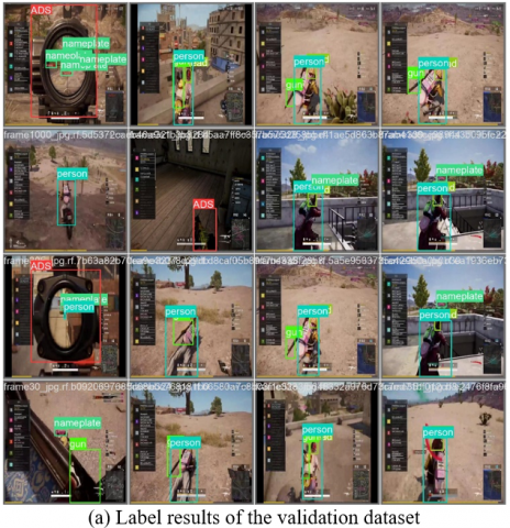
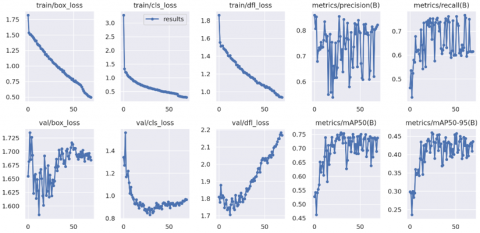
As shown in Figure 8, the labels and predictions of batch 0 in the validation dataset exhibit a high level of synchronization, confirming our outstanding performance in the process of recognizing the dataset. Figure 9 shows the box_loss, cls_loss, and dfl_loss on the training and validation sets. The box_loss calculates the error between the predicted box and the annotated box using Complete Intersection over Union (CIoU). The cls_loss computes whether the anchor box and its corresponding classification are correct, while the dfl_loss represents the distribution focal loss.
mAP50(B) stands for Mean Average Precision at IoU 0.50 for Large Objects, and its formula is as follows:
$m A P=\frac{1}{N} \sum_{i=1}^N A P_i$ (19)
Figure 8. Visualization comparison of batch 0 labels and predictions in the validation dataset
APi refers to the area under the Precision-Recall curve for class i, AP50 signifies that the IoU value is set to 50%, and AP50-95 indicates that the IoU values range from 50% to 95%. The calculation involves taking the mean of the AP values at these IoU levels.
Looking at the convergence curves of the loss functions on the validation set: (1) Box loss, val_loss, and dfl_loss exhibit a trend of initially decreasing and then increasing. Their minimum values appear before training for 50 epochs, suggesting a potential overfitting issue. To address this, it may be beneficial to adjust the learning rate accordingly. (2) Precision fluctuates between 0.5 and 0.8, indicating substantial variability in the model's accuracy. This instability could be attributed to uneven data distribution, and improvements may be achieved by adjusting weights and thresholds. (3) Recall and mAP50 remain relatively stable, maintaining around 0.7. This indicates that the model provides comprehensive coverage of positive samples when identifying targets. (4) mAP50-95 also shows relative stability, hovering around 0.40 with slight fluctuations. This suggests that the model exhibits good robustness and consistent performance on the dataset.
Figure 9. Loss function convergence curve
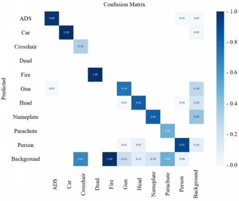
Figure 10 shows the confusion matrix during the prediction process. Each row of this confusion matrix corresponds to the true class, and each column corresponds to the predicted class. Each element in the matrix indicates the percentage of samples belonging to a specific class in the total samples when the model predicts that class.
Figure 10. Confusion matrix
This helps understand the model's classification accuracy for each class and identifies classes that are prone to confusion. Analyzing this confusion matrix allows insights into the model's performance on individual classes and reveals which classes are more likely to be confused. In the graph, it is evident that the confusion probability for the "ADS" class is relatively low, indicating high prediction accuracy. On the other hand, there is a higher confusion probability between the "head" class and the "person" class, possibly due to difficulties in calculating the effective aiming duration and the number of effective aiming instances.
In this study, deep learning visual algorithms were integrated to identify cheating in FPS games, leading to the acquisition of a series of quantifiable player metrics, such as effective aiming duration, through training on key labels. Comprehensive analyses and visualizations of the target detection results were conducted, leading to the conclusion that the model exhibits exceptional performance on crucial labels (such as ADS and nameplate), demonstrating high accuracy. The convergence curves for precision, recall, and F1-Score also indicated favorable performance, providing a reliable basis for subsequent calculations of metrics like effective aiming duration.
Nevertheless, limitations were observed, including notable fluctuations in the precision convergence curve, which suggest issues such as overfitting and potential for improvement in the recognition rate of the "head" label. Future research directions will be aimed at addressing these challenges to further enhance the model's performance. Efforts will be dedicated to finer parameter tuning, with an exploration of more suitable learning rates and adjustment parameters to mitigate model fluctuations and overfitting. To improve recognition of the head label, the introduction of advanced target detection techniques or adjustments to network structures will be considered to better capture features in the head region. Moreover, the ongoing optimization of the dataset, with the incorporation of more gaming scenarios and cheat variations, is aimed at enhancing the model's robustness.
This work was supported by the Industry-University Cooperative Education Project of Ministry of Education of China.
[1] Lugrin, J.L., Cavazza, M., Charles, F., Le Renard, M., Freeman, J., Lessiter, J. (2013). Immersive FPS games: User experience and performance. In Proceedings of the 2013 ACM International Workshop On Immersive Media Experiences, Barcelona, Spain, pp. 7-12. https://doi.org/10.1145/2512142.2512146
[2] Yan, J., Randell, B. (2005). A systematic classification of cheating in online games. In Proceedings of 4th ACM SIGCOMM Workshop on Network and System Support for Games, Hawthorne, NY, USA, pp. 1-9. https://doi.org/10.1145/1103599.1103606
[3] Wu, Y., Chen, V.H.H. (2013). A social-cognitive approach to online game cheating. Computers in Human Behavior, 29(6): 2557-2567. https://doi.org/10.1016/j.chb.2013.06.032
[4] Blackburn, J., Kourtellis, N., Skvoretz, J., Ripeanu, M., Iamnitchi, A. (2014). Cheating in online games: A social network perspective. ACM Transactions on Internet Technology (TOIT), 13(3): 9. https://doi.org/10.1145/2602570
[5] Park, S., Ahmad, A., Lee, B. (2020). Blackmirror: Preventing wallhacks in 3d online fps games. In Proceedings of the 2020 ACM SIGSAC Conference on Computer and Communications Security, Virtual Event, USA, pp. 987-1000. https://doi.org/10.1145/3372297.3417890
[6] Chapel, L., Botvich, D., Malone, D. (2010). Probabilistic approaches to cheating detection in online games. In Proceedings of the 2010 IEEE Conference on Computational Intelligence and Games, Copenhagen, Denmark, pp. 195-201. https://doi.org/10.1109/ITW.2010.5593353
[7] Gaspareto, O.B., Barone, D.A.C., Schneider, A.M. (2008). Neural networks applied to speed cheating detection in online computer games. In 2008 Fourth International Conference on Natural Computation, Jinan, China, pp. 526-529. https://doi.org/10.1109/ICNC.2008.720
[8] Zhang, Q. (2021). Improvement of online game anti-cheat system based on deep learning. In 2021 2nd International Conference on Information Science and Education, Chongqing, China, pp. 652-655. https://doi.org/10.1109/ICISE-IE53922.2021.00153
[9] Nguyen, T.T., Nguyen, A.T., Nguyen, T.A.H., Vu, L.T., Nguyen, Q.U., Hai, L.D. (2015). Unsupervised anomaly detection in online game. In Proceedings of the 6th International Symposium on Information and Communication Technology, Hue, Viet Nam, pp. 4-10. https://doi.org/10.1145/2833258.2833305
[10] Maario, A., Shukla, V.K., Ambikapathy, A., Sharma, P. (2021). Redefining the risks of kernel-level anti-cheat in online gaming. In 2021 8th International Conference on Signal Processing and Integrated Networks, Noida, India, pp. 676-680. https://doi.org/10.1109/SPIN52536.2021.9566108
[11] Woo, J., Kang, S.W., Kim, H.K., Park, J. (2018). Contagion of cheating behaviors in online social networks. IEEE Access, 6: 29098-29108. https://doi.org/10.1109/ACCESS.2018.2834220
[12] Rogers, J., Aygun, R., Etzkorn, L. (2022). Cheat detection through temporal inference of constrained orders for subsequences. In 2022 IEEE Fifth International Conference on Artificial Intelligence and Knowledge Engineering, Laguna Hills, CA, USA, pp. 45-52. https://doi.org/10.1109/AIKE55402.2022.00014
[13] Dinh, P.V., Nguyen, T.N., Nguyen, Q.U. (2016). An empirical study of anomaly detection in online games. In 2016 3rd National Foundation for Science and Technology Development Conference on Information and Computer, Danang, Vietnam, pp. 171-176. https://doi.org/10.1109/NICS.2016.7725645
[14] Kanervisto, A., Kinnunen, T., Hautamaki, V. (2022). GAN-Aimbots: Using machine learning for cheating in first person shooters. IEEE Transactions on Games, 15(4): 566-579. https://doi.org/10.1109/TG.2022.3173450
[15] Ondras, J., Gunes, H. (2018). Detecting deception and suspicion in dyadic game interactions. In Proceedings of the 20th ACM International Conference on Multimodal Interaction, Boulder, USA, pp. 200-209. https://doi.org/10.1145/3242969.3242993
[16] Park, K., Lee, H. (2008). A taxonomy of online game security. In Encyclopedia of Internet Technologies and Applications, pp. 606-611. https://doi.org/10.4018/978-1-59140-993-9.ch085
[17] Yu, S. Y., Hammerla, N., Yan, J., Andras, P. (2012). A statistical aimbot detection method for online FPS games. In the 2012 International Joint Conference on Neural Networks, Brisbane, QLD, Australia, pp. 1-8. https://doi.org/10.1109/IJCNN.2012.6252489
[18] Yahyavi, A., Huguenin, K., Gascon-Samson, J., Kienzle, J., Kemme, B. (2013). Watchmen: Scalable cheat-resistant support for distributed multi-player online games. In 2013 IEEE 33rd International Conference on Distributed Computing Systems, Philadelphia, PA, USA, pp. 134-144. https://doi.org/10.1109/ICDCS.2013.62
[19] Galli, L., Loiacono, D., Cardamone, L., Lanzi, P.L. (2011). A cheating detection framework for unreal tournament iii: A machine learning approach. In 2011 IEEE Conference on Computational Intelligence and Games, Seoul, Korea (South), pp. 266-272. https://doi.org/10.1109/CIG.2011.6032016
[20] Spijkerman, R., Marie Ehlers, E. (2020). Cheat detection in a multiplayer first-person shooter using artificial intelligence tools. In Proceedings of the 2020 3rd International Conference on Computational Intelligence and Intelligent Systems, Tokyo, Japan, pp. 87-92. https://doi.org/10.1145/3440840.3440857
[21] Liu, D., Gao, X., Zhang, M., Wang, H., & Stavrou, A. (2017e). Detecting passive cheats in online games via performance-skillfulness inconsistency. In 2017 47th Annual IEEE/IFIP International Conference on Dependable Systems and Networks, Denver, CO, USA, pp. 615-626.
[22] Su, Y., Yao, D., Chu, X., et al. (2022). Few-shot learning for trajectory-based mobile game cheating detection. In Proceedings of the 28th ACM SIGKDD Conference on Knowledge Discovery and Data Mining, Washington, DC USA, pp. 3941-3949. https://doi.org/10.1145/3534678.3539157
[23] Tao, J., Xu, J., Gong, L., Li, Y., Fan, C., Zhao, Z. (2018). NGUARD: A game bot detection framework for NetEase MMORPGs. In Proceedings of the 24th ACM SIGKDD International Conference on Knowledge Discovery & Data Mining, London, UK, pp. 811-820. https://doi.org/10.1145/3219819.3219925
[24] Xu, J., Luo, Y., Tao, J., Fan, C., Zhao, Z., Lu, J. (2020). Nguard+ an attention-based game bot detection framework via player behavior sequences. ACM Transactions on Knowledge Discovery from Data (TKDD), 14(6): 65. https://doi.org/10.1145/3399711
[25] Jonnalagadda, A., Frosio, I., Schneider, S., McGuire, M., Kim, J. (2021). Robust vision-based cheat detection in competitive gaming. Proceedings of the ACM on Computer Graphics and Interactive Techniques, 4(1): 7 https://doi.org/10.1145/3451259
[26] Han, M.L., Kwak, B.I., Kim, H.K. (2022). Cheating and detection method in massively multiplayer online role-playing game: Systematic literature review. IEEE Access, 10: 49050-49063. https://doi.org/10.1109/ACCESS.2022.3172110
[27] Islam, M.S., Dong, B., Chandra, S., Khan, L., Thuraisingham, B. (2020). GCI: A GPU-based transfer learning approach for detecting cheats of computer game. IEEE Transactions on Dependable and Secure Computing, 19(2): 804-816. https://doi.org/10.1109/TDSC.2020.3013817
[28] Tao, J., Xiong, Y., Zhao, S., et al. (2022). Explainable AI for cheating detection and churn prediction in online games. IEEE Transactions on Games, 15(2): 242–251. https://doi.org/10.1109/TG.2022.3173399
[29] Kaiser, E., Feng, W.C., Schluessler, T. (2009). Fides: Remote anomaly-based cheat detection using client emulation. In Proceedings of the 16th ACM conference on Computer and communications security, Chicago Illinois, USA, pp. 269-279. https://doi.org/10.1145/1653662.1653695
[30] Tao, J., Xiong, Y., Zhao, S., Xu, Y., Lin, J., Wu, R., Fan, C. (2020). Xai-driven explainable multi-view game cheating detection. In 2020 IEEE Conference on Games, Osaka, Japan, pp. 144-151. https://doi.org/10.1109/CoG47356.2020.9231843