Purude Vaishali Narayanrao![]() | Kshiraja Kohirker
| Kshiraja Kohirker![]() | Tadakamalla Shyam Preeth
| Tadakamalla Shyam Preeth![]() | P Lalitha Surya Kumari*
| P Lalitha Surya Kumari*![]()
© 2024 The authors. This article is published by IIETA and is licensed under the CC BY 4.0 license (http://creativecommons.org/licenses/by/4.0/).
OPEN ACCESS
In the field of mental health diagnostics, the acoustic characteristics of speech have been recognized as potent markers for the identification of depressive symptoms. This study harnesses the power of transfer learning (TL) to discern depression-related sentiments from speech. Acoustic features such as rhythm, pitch, and tone form the core of this analysis. The methodology unfolds in three distinct phases. Initially, a Multi-Layer Perceptron (MLP) network employing stochastic gradient descent is applied to the RAVDESS dataset, yielding an accuracy of 65%. This finding catalyzes the second phase, wherein a comprehensive hyperparameter optimization via grid search (GS) is conducted on the MLP Classifier. This step primarily focuses on detecting emotions commonly associated with depression, including neutrality, sadness, anger, fear, and disgust. The optimized MLP classifier indicates an improved accuracy of 71%. In the final phase, to enhance precision further, the same GS-based model, underpinned by TL principles, is applied to the TASS dataset. This application astonishingly achieves an accuracy of 99.80%, suggesting a high risk of depression. This comparative study establishes the proposed framework as a vanguard in the application of TL for depression prediction, showcasing a significant leap in accuracy over previous methodologies.
depression, transfer learning (TL), grid search (GS), speech analysis, Multi-Layer Perceptron (MLP) classifier
Predictive modeling uses statistics and machine learning algorithms to create models that can perfectly predict future events or behaviors. In healthcare, predictive modeling can identify patients at risk of developing certain diseases or conditions, predict the outcomes of medical interventions, and improve patient outcomes by providing personalized treatment plans [1-3].
The methodology for developing predictive models in healthcare involves several steps, including problem definition, dataset preparation, pre-processing of data, selecting an apparent model, training the model, and performance evaluation of the model [4-7]. Factors that can affect the performance of predictive models include the size of the dataset and its quality, which is used to train the model, the choice of modeling algorithm, and the tuning of model parameters.
According to the World Health Organization (WHO), a healthy person possesses a healthy brain along with physical wellness. To diagnose depression, different treatment techniques include medication, meditation, and psychotherapy. For creating an efficient and practical system to predict depression Vocal and visual data keys can be easily captured using a microphone and camera. This approach is convenient for collecting data when it is compared with sensors, as they need to be attached physically to the person, for example, ECG and EEG data. It is also difficult for machines to capture this data in an environment that is not controlled.
The neural network model has shown good results in stress prediction. They are powerful models that have proven effective in text classification, image, and signal processing tasks, as well as in NLP (natural language processing). MLP classifiers can be a better approach for predicting depression in humans using speech signals. They can learn essential elements from raw data, such as physiological signals or text, without relying on handcrafted features [8-10].
This is particularly relevant for depression prediction, where relevant features may not be immediately apparent or vary across individuals. Furthermore, MLP classifiers can handle complex data structures, such as time-series or multi-channel data, often encountered in depression prediction tasks. For example, speech recordings are often used to assess stress levels.
1.1 Challenges for speech-based depression prediction
Uncompressed audio in the WAV format is stored as a series of numerical values that represent the intensity of the recorded sound pressure at each moment in time. Within the WAV standard, these integers are compressed into a sequence of bytes. The understanding of this sequence of bytes relies on two primary components. The first factor to consider is the sampling rate, typically measured in hertz, which represents the number of samples per second in our audio data. The second parameter is the sample width, which represents the number of bits used for each sample (also known as the bit rate). The header of each WAV file contains several parameters, including the number of channels (mono or stereo) and other relevant parameters. Frames typically contain a complete byte sequence that represents all the audio samples in a sound file. Our objective entailed decomposing a byte string for each file into an array of numerical values that could be subjected to further analysis.
1.2 Existing methods
Quatieri and Malyska [11] proposed that voice quality measures commonly employed in depression detection can be adopted from signal-processing techniques. Some of these measurements are jitter, shimmer, harmonic-to-noise ratio, small changes in glottal pulse amplitude within voiced regions, and the ratio of harmonics to inharmonic components. These characteristics were associated with the oscillation of the vocal folds, which was affected by the tension of the vocal folds and the pressure below the vocal cords. The study found that there is a connection between laryngeal biomarkers and psychomotor retardation assessment. This connection helps us better understand the neurophysiological reasons behind changes in voice quality during depression and the deterioration of human speech.
Due to its objective advantage and easy-to-acquire nature, voice data has gained attention. The voice of a depressed person possesses characteristics like a low speech rate, many pauses, a lack of confidence, and more use of negative words. The speech of the depressive subject is spiritless, uninteresting, and monotone. These changes in acoustic features are used in machine learning algorithms for the prediction of depression risk.
In this research article, experiments are performed on the RAVDESS dataset and the TASS dataset [12] using a MLP classifier. Experiments are performed in the following 3 steps:
(1) Apply MLP to the RAVDESS dataset.
MLP means the MLP Network, which uses both feed-forward and backpropagation in Artificial Neural Network (ANN). It suits large, non-linear datasets with good performance. MLP uses back propagation by calculating the partial derivative of the loss function at each time stamp. Hence, the model is trained iteratively. It avoids overfitting by using regularization.
(2) Apply GS on RAVDESS using optimized hyperparamers.
GS identifies the best hyperparameters for hidden layers, activation function, and solver. These parameters are provided in a dictionary, using which a GS identifies the best estimator. Once the GS is fitted to the training data, we can find the parameters that resulted in the highest score. GS improves the performance of the model by providing optimized parameters.
(3) Transfer the learning of the model in step 2 to the new dataset, TESS.
TL is an approach in which a model is trained and used as the basis for the target task. To transfer knowledge from one model to another, a TL approach is used in machine learning and deep learning. It can be applied using several strategies, such as whether to transfer the whole model to a new target dataset or use part of the model. It is mainly used to save resources and improve efficiency, like a human being. It is used in many applications, including speech and emotion recognition. Research is carried out for traffic anomaly detection using TL and fuzzy systems [13].
The novel contribution of the proposed research is as follows: A framework is proposed for predicting depression symptoms that accepts an audio file representing the speech of a depressed person and uses the librosa module to convert audio files to digital data. The first MLP classifier is used to identify the symptoms, and then, using GS on hyperparameters, the same process is repeated. An improvement in performance is observed.
MLPs can learn to extract meaningful patterns from these signals by taking vectors as input. Another advantage of MLPs is their ability to handle missing values and noisy data. This is especially important in depression prediction, where data may need to be completed or be subject to measurement errors. MLPs can learn to tolerate such imperfections and still make accurate predictions. Lastly, MLPs can handle large, complex datasets often required for reliable prediction. This is important because stress levels indicating depression vary widely across individuals and may depend on factors such as age, gender, or occupation. Using a deep TL approach, the optimized model is applied to a new dataset to improve efficiency.
The research paper is divided as follows: Section II performs a survey on related work in this area. Section III provides a description of the proposed framework, and Sections IV and V display and discuss the experimental results. Section VI compares and analyzes the research work, while Section VII concludes the paper.
Automatic depression prediction is currently a rapidly growing research domain. After surveying 15-20 papers from past years, related work using audio signals was found in the following literature survey on verbal clues:
Using speech as input, research is being carried out in this area for stress emotion recognition in speech [14-16]. The authors [17] proposed an artificial intelligence (AI) system that gives a scale for automatic depression prediction. In the research, vocal expressions are obtained using spectral descriptors and Mel-frequency cepstral coefficient (MFCC) features from audio data. The dataset used for this task is Audio/Visual Emotion Challenges 2014. The classifier used is logistic regression. While the authors [18] used binary logistic regression to detect a relationship between voice and depression, The authors [19] improved the accuracy of the base classifier Logistic Regression for better classification by using an ensemble technique. In the experiment the author conducted [20], data was inputted to CNN by converting audio to images.
Speech recognition is useful in many domains, like security and the speech-controlled home mechanization framework [21]. The voice of a person is a valuable biometric feature and can be used for identity verification [22]. But the available dataset should be noise-free for better prediction accuracy. Hence, some authors have done research to enhance the quality of speech signals using sparse representation and dictionary learning [23]. Speech signals can also be used for speech-sound disorder recovery in child patients. It may be applicable for languages like Telugu [24].
Due to the limitations of traditional machine learning algorithms, the author has researched how features can be extracted from abnormal speech and can be related to the mental state of the patient. And implemented bidirectional CNN using a hidden emotion vector [25]. While some authors have used ensemble CNN by averaging the results of multiple CNNs for automatic depression detection in speech [26], Some researchers have assessed depression levels in speech using spectrogram-based CNN [27].
Depression's impact on paralinguistic speech characteristics and the utilization of this knowledge in classification and prediction systems have been explored by numerous researchers [28]. These linkages show great potential for quantification through automatic depression detection (ADD) systems. The 2017 AVEC "Real-life Depression and Affect Recognition Workshop and Challenge" held by the Association for Computing Machinery [29] placed significant emphasis on the scientific examination of depression. During the conference, Yang et al. [30] presented a hybrid multi-modal framework for recognizing and classifying depression. The framework consists of three sections: predicting the patient health questionnaire depression scale (PHQ-8) [31] score using audio and video features; classifying depression or non-depression based on text information; and using multimodal regression to make the final depression prediction. The method did a better job of estimating the PHQ-8 score than the baseline results, as shown by the mean absolute error (MAE) [32] and the root-mean-square error (RMSE). The MAE was 4.359, and the RMSE was 5.400. The remaining outcomes were also gratifying. The utilization of paragraph vectors and support vector machine (SVM) models for text-based categorization resulted in accuracies of 84.21% for female participants and 81.25% for male subjects [33]. Yang et al. [34] introduced a multi-modal fusion architecture consisting of deep convolutional neural network (CNN) models [35]. Their approach incorporated audio, video, and text streams and achieved superior performance compared to the baseline in predicting PHQ-8 scores using audio, video, and text data (with a mean absolute error of 3.980 and a root mean square error of 4.653). Additional intriguing findings were reported at the 2018 Interspeech Conference. Afshan et al. [36] specifically examined the efficacy of voice quality characteristics in identifying depression. The writers suggested using voice quality parameters along with MFCCs [37], which would make depression detection more accurate. Consequently, they managed to attain a precision rate of 77%, even when the test utterances were as brief as 10 seconds.
Table 1. Study of existing methodology on detecting depression using GS
|
S.No. |
Author and Year |
Methodology |
Dataset |
Remark |
|
1 |
Wang et al. [25], 2021 |
bidirectional CNN |
DAIC-ori |
Accuracy = 74.29% Precision = 58.33% F1 Score = 60.9% |
|
2 |
Vázquez-Romero and Gallardo-Antolín [26], 2020 |
Ensembled CNN |
AVEC-2016 |
Accuracy = 72% Precision = 52% F1 Score = 63% Recall = 79% |
|
3 |
Srimadhur and Lalitha [27], 2020 |
End to end CNN |
AVEC-2016 |
Accuracy = 61.32% Precision = 58% F1 Score = 66% Recall = 77% |
|
4 |
Muslim [38], 2020 |
SVM Optimization using GS |
Amazon review |
Accuracy = 80.8% |
|
5 |
Garain et al. [39], 2020 |
SVR and GS |
|
Precision = 66% F1 Score = 67% Recall = 66.33% |
|
6 |
Sandhu et al. [40], 2023 |
EmbedLSTM |
Product Review |
Accuracy = 95.55% Precision = 97.61% F1 Score = 97.42% Sensitivity = 97.23% Specificity = 84.91% |
|
7 |
Elgeldawi et al. [41], 2021 |
Bayesian Optimization |
Arabic |
Accuracy = 95% |
|
8 |
Sumathi [42], 2020 |
Random forest and GS |
Customer feedback data |
Recall = 96.13% Precision = 85.93% F1 Score = 90.74% Sensitivity = 96.13% Specificity = 84.26% |
|
9 |
Priyadarshini and Cotton [43], 2021 |
GS-based DNN |
IMDB |
Accuracy = 97.8% Precision = 98.2% F1 Score = 97.2% Sensitivity = 98.9% Specificity = 99% |
Since the last two to three decades, researchers have been using machine learning in various areas, including predictive analytics. But limited researchers have focused especially on depression level prediction using the GS technique on acoustic signals. Table 1 indicates the study of existing methods for GS.
From this survey, it is observed that while detecting depression using audio files as input, the GS-based TL approach is not used to get a model with improved accuracy. This is the first effort that shows improvement in accuracy after using GS and deep TL based on acoustic features of speech.
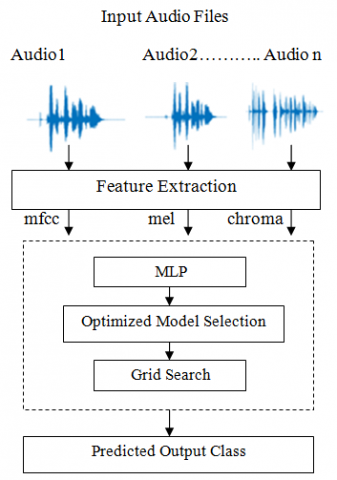
The system architecture proposed for research is as shown in Figure 1, which uses the RAVDESS dataset and GS. We will load the data by reading the audio dataset, then extract the above features from it and determine dependent and independent data. Next, get training and testing sets by splitting the dataset and initializing the parameters for the MLP classifier to train the model. At the end, evaluate the model by calculating the accuracy and analyzing the performance of the classifier.
Figure 1. System architecture
The observed accuracy is not satisfactory; hence, optimization is done using hyperparameters for GS. The model is again trained and tested. An improvement in accuracy of up to 71% is observed.
The process for identifying depression symptoms using speech signals is proposed using the following steps:
3.1 Load the speech dataset
Depression symptoms identification using audio datasets RAVDESS and TESS. The datasets are available freely to the public and contain audio files without any background noise. This has the advantage of improving the accuracy of the model.
For the research, the audio datasets used are:
RAVDESS is the Ryerson Audio-Visual Database of Emotional Speech dataset [44]. It contains 7356 files of 247 individuals with different emotions, intensity, and genuineness. The size of the dataset is 24.8GB.
The RAVDESS dataset includes the following data fields:
TESS is the Toronto emotional speech set dataset [12]. It contains 2800 speech files and different emotions such as sadness, anger, fear, disgust, happiness, pleasant surprise, and neutral for each of them.
Two actresses, aged 26 and 64, recited a set of 200 target phrases in the carrier phrase "Say the word _____." Recordings were taken of the set, with each word being portrayed in seven different emotions: anger, disgust, fear, happiness, pleasant surprise, sadness, and neutral. The total number of stimuli is 2800. Two actresses were enlisted from the Toronto region. Both actresses are native English speakers, hold university degrees, and have received musical education. Both actresses' audiometric testing revealed thresholds that fall within the usual range.
3.2 Preprocessing
(1) Feature Extraction (Mel, MFCC, Chroma, ZCR, and RMS)
Librosa is the main library used, along with Pyaudio and Soundfile. In Python, the Librosa library is used to analyze music and audio. It is backward compatible in terms of code readability and modularity. Sklearn is also used to build a model using MLP classifier for emotion recognition using sound files.
The Librosa module is used to convert inputted audio files to digital data. Librosa uses the Mel, MFCC, Chroma, ZCR, and RMS features for this conversion. MFC plays a major role in emotion recognition from speech signals [45]. Mel captures the frequency of the signal represented on the Mel scale, MFCC describes the short-term spectrum of an audio file, the Chroma feature captures harmonic and melodic characteristics based on the pitch of the audio file, ZCR represents the rate of sign changes in the signal for the particular frame, and RMS analyzes the changes in the loudness to extract features from a new audio file.
(2) Relevant feature selection
Emotional features present in the audio dataset are pitch, energy, loudness, and rhythm. Acoustical information is obtained from these during a preprocessing technique called feature extraction. The Librosa module is used to convert data from an audio file into digital form using features such as Mel, MFCC, Chroma, ZCR, and RMS. These speech features contain necessary information that helps with the classification.
3.3 Set the hyperparameters required for GS
Hyperparameter optimization is a technique that involves searching through a range of values to find a subset of results that achieve the best performance on a given dataset. When performing hyperparameter optimization, we first need to define a parameter space or parameter grid, where we include a set of possible hyperparameter values that can be used to build the model. The GS technique is then used to place these hyperparameters in a matrix-like structure, and the model is trained on every combination of hyperparameter values. The model with the best performance is then selected.
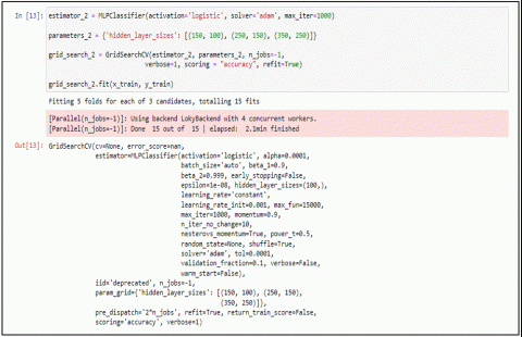
The hyperparameters are required to obtain the optimum performance of the architecture. The optimized values of these hyperparameters are mentioned in Table 2 and implemented in experiments as shown in Figure 2.
Table 2. Details of GS hyperparameters
|
Parameter Name |
Values |
|
Activation Function |
logistic |
|
Solver |
Adam |
|
Max_iterations |
1000 |
|
Hidden Layer Sizes |
(150,100),(250,150),(350,250) |
|
Evaluation paramter |
Accuracy |
|
Learning rate |
0.001 |
|
Batch_size |
auto |
By default, MLP has three hidden layers.
The activation function for the hidden layer used for hidden layers is logistic, which means the logistic sigmoid function returns f(x) = 1/(1+exp(-x)).
For weight optimization, the Adam solver is used. It refers to a Stochastic Gradient-Descent (SGD)-based optimizer. Adam is a perfect solver for datasets with large training samples. It is efficient for both the training and validation phases. SGD updates the weight parameters after each individual training sample. It is faster and can handle large datasets.
Batch_size, when set to "auto," is calculated as min(200,n,samples).
Learning rate determines weight update schedule. The constant value indicates that the learning rate is given by the parameter ‘learning_rate_init’. Its value is 0.001. During weight updation, step size is controlled by the learning rate. This rate is applicable only for Adam Solver with SGD Optimizer.
The maximum number of iterations iterated by the solver is indicated by Max_iterations. It indicates the epoch value for stochastic solvers like SGD or Adam. Epoch means the number of times each data point is used.
3.4 Split the dataset into training and testing sets
The used dataset should be divided into training and testing sets. In machine learning, it’s a crucial step. The model learns from the training set and applies the learned knowledge to the testing set (unknown data). The accuracy at this stage assesses the performance of the model.
3.5 Apply the MLP classifier and train the model
Using MLP, the output is predicted for each sentiment class in the set. The set contains five classes: angry, disgusted, fearful, neutral, and sad. Each of these sentiments is related to depression and can be considered a depression symptom. Hence, if the sentiment of the input audio indicates any of the above sentiments, then the audio indicates the risk of depression.
A neural network is a replica of the human brain with multiple interconnected neurons. The neural network works on a function that uses a scalar product, which is the product of input with weight.
f(x,w)=x1w1+….xnwn (1)
Figure 2. GS hyperparameters
where, xi is input and wi is weight. The neuron is known as the perceptron, as it performs a human brain-like function of perception. The perceptron is a basic unit of computation that relies on weighted sums, as shown in Eq. (1). Perceptron combines input into a weighted sum, and when the sum crosses the threshold, it fires output.
$y=\{\begin{matrix}
\text{Weighted} \\
1,\text{ }\!\!~\!\!\text{ if }\!\!~\!\!\text{ }{{\sum }_{\text{i}}}{{\text{w}}_{\text{i}}}{{\text{x}}_{\text{i}}}\text{ }\!\!~\!\!\text{ T}>~0 \\
0,\text{otherwise} \\
\end{matrix}$ (2)
If the weighted sum is greater than the threshold, then it gives the output as 1, otherwise 0 as illustrated in Eq. (2). Such perceptron is applicable for classification tasks. The difference between misclassified data and target data is called loss. To minimize this loss, the optimization function used is stochastic gradient descent. The last function used is the activation function, which can make the decision on the activation of a neuron whether it will fire or not.
A MLP has stacked neurons arranged in layers named input layers, output layers, and one or more hidden layers. In MLP, the neuron can use any activation function arbitrarily. In the model, the logistic sigmoid function is used as an activation function. The sigmoid function returns an s-shaped curve, whereas in the logistic sigmoid function, the return value varies between 0 and 1 instead of -1 and 1. The logistic sigmoid function is given in Eq. (3).
f(x)=1/1+e-x (3)
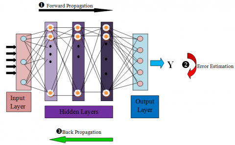
The MLP model is shown in Figure 3.
Figure 3 represents MLP models consisting of an input layer, three hidden layers, and an output layer. The features extracted from the audio dataset act as input. The result obtained from computations of input xi and weight wi is propagated to hidden layers in a forward direction; hence, it is also called a feed-forward network (step 1 in Figure 3). Using the activation function, the results of the hidden layer are forwarded as output. Error estimation means the loss calculation (step 2 in Figure 3).
Loss is defined as the difference between targeted output and obtained output. The model is said to be accurately trained or learned when it has a negligible error function. Weight plays a crucial role in learning. Hence, the model has to find the correct weights to minimize the loss. The model has to undergo multiple iterations to get trained. Using the backpropagation algorithm, the model adjusts weights in the network, keeping the goal of the minimum loss function (step 3 in Figure 3).
Backpropagation relies on gradient descent as an optimization function. The weight update process includes propagation in a backward direction from hidden layers to the input layer to minimize the error given by Eq. (4). The weights in the next timestamp depend on the previous timestamp to reduce errors.
$\Delta w\left( t \right)=-\in \frac{dE}{dw\left( t \right)}+\propto \Delta w\left( t-1 \right)$ (4)
The backpropagation algorithm [46, 47] runs through three phases:
Phase 1: Feed-forward phase
This phase propagates from the input layer to the output layer by calculating the weighted sum and applying the activation function.
Phase 2: Back-propagation phase
The exact reverse of phase 1 is backpropagation, which moves from the output layer to the input layer. After calculating the loss function at the output layer, phase 2 updates weights using Eq. (4).
Phase 3: Global Error Phase
This concluding phase finds the effect of weight adjustment using backpropagation on the loss.
3.6 Test the model on a test set
In addition to training, testing is also a crucial step in machine learning. As the dataset is divided into a training set and a testing set, this step evaluates the performance of the model on unseen data in the testing set. The model is learned when it achieves better accuracy during the testing phase. The model is called generalized and is trained for real-world problems.
Figure 3. Back propagation in MLP
3.7 Evaluate the model using evaluation metrics such as accuracy, precision, recall, and F1-score
In the first step, MLP is applied to RAVDESS, and the observed accuracy is 65%. Hence, in the next step, parameter sweep, that is, hyperparameter optimization, is achieved via GS on the MLP classifier to find the best hyperparameters. Some emotions, such as 'neutral', 'sad', 'angry’, 'fear', and 'disgust', are common symptoms of depression. Using the MLP classifier, these emotions can be identified with an accuracy of 71%. Using the TL approach, the same exhaustive GS-based model is applied to the TASS dataset and observed 99.80% accuracy, which indicates that person may be at high risk of depression.
Table 3. GS and TL algorithms
|
Algorithm 1: GS Algorithm |
|
Input: RAVDESS dataset |
|
Begin Steps:
End |
|
Output: Prediction of depression symptoms. |
|
Algorithm 2: TL Algorithm |
|
Input: TESS dataset and pre-trained model from GS algorithm |
|
Begin Steps:
End |
|
Output: Improved Prediction of depression symptoms. |
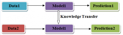
Figure 4. TL
To identify emotions indicating depression symptoms, the MLP classifier is used. That is the MLP classifier, which uses stochastic gradient descent for optimizing the log-loss function. The MLP classifier uses a feed-forward artificial neural network. Table 3 indicates the algorithm to implement MLP with GS.
Algorithm 1 is named as GS. The algorithm applies GS to the RAVDESS dataset; hence, the input to the algorithm is noise-free audio files in the RAVDESS dataset. The libraries required for experimentation are librosa, soundfile, and sklearn; hence, they are installed. After reading audio files, feature extraction is done using the soundfile library. After finding dependent and independent features, the dataset is divided into training sets (75%), and testing sets (25%). As the model uses MLP, hyperparameters required for MLP are specified and GS is applied. The performance metrics model is evaluated.
TL means imposing the knowledge acquired during training one model on a particular task and applying the same model to a different and related task. It is reusing the model and gaining the advantage of performance improvement. It saves time in training the model from scratch. The main advantages of TL are faster training and improved generalization. TL involves leveraging knowledge acquired from one activity to enhance the ability to generalize in another one. We move the learned weights from "task A" to a new "task B" in the network. The fundamental concept is to leverage the acquired knowledge of a model from a task with ample labeled training data to tackle a new problem that lacks sufficient data. Rather than commencing the learning process from the beginning, we initiate it by utilizing patterns acquired from accomplishing a task that is connected. TL is mostly employed in computer vision and natural language processing tasks, such as sentiment analysis, due to the substantial computational resources needed. It has become highly relevant when used in conjunction with neural networks that necessitate substantial quantities of data and computational capacity. TL involves utilizing the early and middle layers while only retraining the latter layers. It assists in utilizing the annotated data from the original training activity.
In this research using the TL technique, the model that has already been trained using the RAVDESS dataset is applied to the TESS dataset, and an improvement in accuracy is observed. The knowledge transfer from the same base model to different datasets is known as TL. It is indicated in Figure 4.
Table 3 also indicates the TL algorithm on the TESS dataset. As a trained model is available with hyperparamters, the only change in algorithm 2 is the input dataset, which is TESS. When MLP with GS is applied to TESS, a significant change in accuracy is observed. This is the main advantage of TL: as the model is trained, accuracy is improved, and a generalized model is obtained.
Accuracy is a sufficient metric to evaluate the performance of the classification task on a balanced dataset. As both datasets used in the research are inbalanced (all classes are not equal in numbers), it needs additional metrics like recall, precision, and F1-score to evaluate the model's performance. All the metrics use true positive (TP), true negative (TN), false positive (FP), and false negative (FN).
TP indicates how correctly positive samples are classified.
TN indicates how correctly negative samples are classified.
EP indicates how incorrectly positive samples are classified.
FN indicates how incorrectly negative samples are classified.
The performance metrics used for valuation is indicated using Eqs. (5)-(8).
Accuracy= TP+TN / TP+TN+FP+FN (5)
Precision= TP / TP+FP (6)
Recall= TP / TP+FN (7)
F1= 2(Precision*Recall) / (Precision+Recall) (8)
The performance of both algorithms, GS and TL, is evaluated using a confusion matrix and classification report.
Confusion Matrix: The table that evaluates the performance of the classification task is the Confusion Matrix. The target labels are compared with the predicted labels. It provides a detailed view of the classification and accuracy of the model for all classes. When the class distribution in a given dataset is imbalanced, the confusion matrix is the tool to assess the performance of the model. It is represented in Table 4.
Classification Report: The classification summary after the evaluation of the model is given by the classification report. By using the information in the confusion matrix, it defines evaluation metrics like precision, recall, F1 score, accuracy, and support for all the classes. These parameters are defined using Eqs. (5) and (8). Support specifies the number of instances in the dataset that belong to a specific class. The Classification Report is a useful tool for multi-class classification (more than two classes). It identifies how correctly each class is predicted by the model.
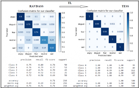
Figure 5 indicates results after executing algorithms 1 (GS) and 2 (TL). The results are displayed using the Confusion Matrix and Classification Reports for both datasets, RAVDESS and TESS. Algorithm 1 (GS) is applied to the RAVDESS dataset, and Algorithm 2 (TL) is applied to the TESS dataset. For GS, precision ranges from 52 to 75%, F1-score ranges from 52 to 78%, and accuracy is 71%. For TL, all metrics—precision, recall, F1-score, and accuracy—range from 99 to 100%.
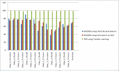
Table 5 shows the results obtained by each class (anger, sadness, disgust, neutral, and fearful) in all 3 phases of the experiment. The phases are experiments performed on the RAVDESS dataset using an MLP classifier and without GS. The second phase of the experiment is on the same RAVDESS dataset using GS. And in the third phase, experiments are carried out using the same trained model for different datasets (TESS. The evaluation parameters used are precision, recall, F1 score, and accuracy. The corresponding plot is shown in Figure 6.
Table 4. Confusion matrix
|
|
Predicted Positive |
Predicted Negative |
|
Actual Positive |
TP |
FN |
|
Actual Negative |
FP |
TN |
Figure 5. Confusion matrix and classification report for TL from RAVDESS to TESS
Figure 6. Results of 3 phases
The values in Table 5 clearly indicate that when no hyperparameter optimization is applied and only an MLP classifier is used on the RAVDESS dataset, the sentiments of five classes are classified with a poor accuracy of 65 to 68%. Even precision, recall, and F1 scores are also poor. A slight improvement is observed when parameter tuning is performed on the same classifier with the same input dataset. Extremely high improvements in accuracy are observed when TL is applied to the trained model and the dataset is changed to TVSS. All the evaluation metrics using both techniques (GS and TL) achieve performance of more than 98%. The findings highlight the potential of TL as a powerful approach for improving the prediction of depression using sentiment analysis on audio data. The improvement in accuracy obtained is highlighted by the green color in the graph shown in Figure 6.
Table 5. Evaluation metrics of 3 phases
|
Sentiment Class Representing Depression Symptom |
RAVDESS Using MLP (No Grid Search) |
RAVDESS Using Grid Search on MLP |
TESS Using Transfer Learning |
|
Class-0-Precision |
79 |
75 |
100 |
|
Class-0-Recall |
76 |
80 |
100 |
|
Class-0-F1 Score |
78 |
78 |
100 |
|
Class-1-Precision |
66 |
76 |
98 |
|
Class-1-Recall |
90 |
79 |
100 |
|
Class-1-F1 Score |
76 |
77 |
99 |
|
Class-2-Precision |
78 |
67 |
100 |
|
Class-2-Recall |
49 |
74 |
99 |
|
Class-2-F1 Score |
60 |
70 |
100 |
|
Class-3-Precision |
67 |
52 |
100 |
|
Class-3-Recall |
38 |
52 |
98 |
|
Class-3-F1 Score |
48 |
52 |
99 |
|
Class-4-Precision |
57 |
72 |
99 |
|
Class-4-Recall |
66 |
58 |
100 |
|
Class-4-F1 Score |
61 |
64 |
100 |
|
Accuracy |
68 |
71 |
99 |
Figure 7. Comparative analysis for proposed work using transfer leaning
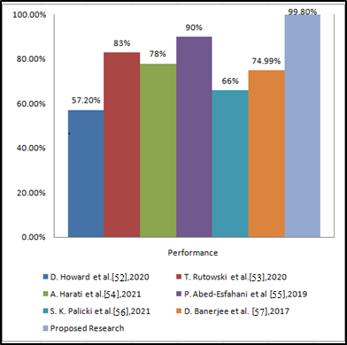
The proposed model is analyzed by comparing the previous work using TL and the same dataset, RAVDESS and TESS. Table 6, Table 7, and Table 8 show the comparative study. A comparative analysis of the proposed model with speech-emotion classification (Table 6), GS (Table 7), and TL (Table 8) techniques is taken into consideration. According to analysis, it is observed that when MLP is applied to the RAVDESS dataset for depression-related emotion classification using the speech dataset, the observed accuracy is poor, at only 65%. Then, in the next phase of the experiment, hyperparameters are defined and GS on the same dataset is applied. The accuracy of the classification task has improved from 65% to 71%. But still, the accuracy obtained is not satisfactory. Hence, a trained model is applied to a similar type of dataset, which is TESS. When TL was used by other researchers in the past, the observed accuracy was only 52% to 90%. But in the proposed research, an observable accuracy of 99.8% is obtained. The graphical representation of the comparative analysis in Table 8 is shown in Figure 7.
Table 6. Speech emotion classification
|
S.No. |
Author and Year |
Methodology |
Dataset |
Performance |
|
1 |
Negi et al. [48], 2018 |
CNN |
DAIC-WOZ |
93% (F1-score) |
|
2 |
Muslim [38], 2020 |
LSTM |
MHMC emotion database and CHI-MEI mood database |
73.33% (Acc) |
|
3 |
Poojary et al. [49], 2021 |
MLP |
RAVDESS |
100% (Acc) |
|
4 |
Vamsi et al. [50], 2021 |
CNN |
RAVDESS,TESS,SAVEE |
83.32 (Acc) |
|
5 |
Idris et al. [51], 2015 |
MLP |
Berlin Emotional Database |
78.69% (Acc) |
|
6 |
Proposed Research |
MLP |
RAVDESS |
65% (Acc) |
Table 7. GS-based models
|
S.No. |
Author and Year |
Methodology |
Dataset |
Performance |
|
1 |
Wang et al. [25], 2021 |
bidirectional CNN |
DAIC-ori |
Accuracy = 74.29% |
|
2 |
Vázquez-Romero and Gallardo-Antolín [26], 2020 |
Ensembled CNN |
AVEC-2016 |
Accuracy = 72% |
|
3 |
Srimadhur and Lalitha [27], 2020 |
End to end CNN |
AVEC-2016 |
Accuracy = 61.32% |
|
4 |
Muslim [38], (2020) |
SVM Optimization using GS |
Amazon review |
Accuracy = 80.8% |
|
5 |
Garain et al.[39], 2020 |
SVR and GS |
|
F1 Score = 67% |
|
6 |
Sandhu et al.[40], 2023 |
EmbedLSTM |
Product Review |
Accuracy = 95.55% |
|
7 |
Elgeldawi et al. [41], 2021 |
Bayesian Optimization |
Arabic |
Accuracy = 95% |
|
8 |
Sumathi et al. [42],2020 |
Random forest and GS |
Customer feedback data |
F1 Score = 90.74% |
|
9 |
Priyadarshini and Cotton [43], 2021 |
GS based DNN |
IMDB |
Accuracy = 97.8% |
|
10 |
Proposed Research 2023 |
GS based MLP |
RAVDESS |
Accuracy = 71% |
Table 8. TL-based models
|
S.no. |
Author and Year |
Methodology |
Dataset |
Performance |
|
1 |
Howard et al. [52], 2020 |
AutoML |
Australian mental health peer-support forum Reachout.com and UMD Reddit Suicidality Dataset |
57.20% (F1-score) |
|
2 |
Rutowski et al. [53], 2020 |
NLP |
Speech dataset collected by Ellipsis health |
83% (AUC) |
|
3 |
Harati et al. [54], 2021 |
RecurrentCNN |
Speech dataset collected by Ellipsis health |
78% (AUC) |
|
4 |
Abed-Esfahani et al [55], 2019 |
AutoSkLearn |
University of Maryland (UMD) Reddit Suicidality Dataset |
90% (Recall) |
|
5 |
Palicki et al. [56], 2021 |
LR |
Brexit tweets |
66% (Acc) |
|
6 |
Banerjee et al. [57], 2019 |
Deep Belief Network (DBN) |
Post-traumatic stress disorder patient data from structured interview |
74.99% (Acc) |
|
7 |
Proposed Research |
TL-based MLP |
TESS |
99.8 % (Acc) |
The research proposed a method that uses deep TL to predict the risk of depression using speech datasets. The experiments are carried out on three network architectures, and it is proved that the combination of hyperparameter turning in GS and TL presents highly accurate classification results. A new direction is suggested by the results while using audio data for prescreening depressive people by using their voice. The spectrograms demonstrated the capacity to generate features that can be learned by a MLP. The algorithm achieved accuracies of 99% with the utilization of the TL technique. This occurred in spite of the arduous character of voice as a predicator of depression. The suggested model has the capability to function autonomously or as a component of a more intricate, hybrid, or multimodal solution. The primary benefits of this approach lie in its inherent simplicity, combined with its cutting-edge precision.
In future research, the utilization of TL can be employed on the primary dataset to accurately detect depressive symptoms from speech signals. Using different neural network topologies in multi-modal methods makes them more effective than single-modality methods, which makes them an interesting topic for more research. The proposed model can be utilized as a foundational component for a more intricate, hybrid, or multimodal system designed to identify depression. The proposed approach serves as a novel depression screening tool that benefits both clinical therapists and patients within the community.
[1] Liang, L., Liu, M., Martin, C., Sun, W. (2018). A deep learning approach to estimate stress distribution: A fast and accurate surrogate of finite-element analysis. Journal of the Royal Society Interface, 15(138): 20170844. https://doi.org/10.1098/rsif.2017.0844
[2] Jaques, N., Taylor, S., Sano, A., Picard, R. (2017). Predicting tomorrow’s mood, health, and stress level using personalized multitask learning and domain adaptation. In IJCAI 2017 Workshop on Artificial Intelligence in Affective Computing, 17-33.
[3] Sumathi, V., Velmurugan, R., Sudarvel, J., Sathiyabama, P. (2021). Intelligent classification of women working in ICT based education. In 2021 7th International Conference on Advanced Computing and Communication Systems (ICACCS), Coimbatore, India, pp. 1711-1715. https://doi.org/10.1109/ICACCS51430.2021.9441803
[4] Kumar, S., Jain, A., Kumar Agarwal, A., Rani, S., Ghimire, A. (2021). Object-based image retrieval using the U-Net-based neural network. Computational Intelligence and Neuroscience, 2021: 4395646. https://doi.org/10.1155/2021/4395646
[5] Kumar, S., Rani, S., Jain, A., Verma, C., Raboaca, M.S., Illés, Z., Neagu, B.C. (2022). Face spoofing, age, gender and facial expression recognition using advance neural network architecture-based biometric system. Sensors, 22(14): 5160. https://doi.org/10.3390/s22145160
[6] Kumar, S., Jain, A., Rani, S., Alshazly, H., Idris, S.A., Bourouis, S. (2022). Deep neural network based vehicle detection and classification of aerial images. Intelligent Automation & Soft Computing, 34(1): 119-131. http://doi.org/10.32604/iasc.2022.024812
[7] Kumar, S., Jain, A., Shukla, A.P., Singh, S., Raja, R., Rani, S., Harshitha, G., AlZain, M.A., Masud, M. (2021). A comparative analysis of machine learning algorithms for detection of organic and nonorganic cotton diseases. Mathematical Problems in Engineering, 2021: 1-18. https://doi.org/10.1155/2021/1790171
[8] Rani, S., Lakhwani, K., Kumar, S. (2022). Three dimensional objects recognition & pattern recognition technique; related challenges: A review. Multimedia Tools and Applications, 81(12): 17303-17346. https://doi.org/10.1007/s11042-022-12412-2
[9] Rani, S., Ghai, D., Kumar, S. (2022). Reconstruction of simple and complex three dimensional images using pattern recognition algorithm. Journal of Information Technology Management, 14: 235-247. https://doi.org/10.22059/jitm.2022.87475
[10] Rani, S., Ghai, D., Kumar, S. (2022). Object detection and recognition using contour based edge detection and fast R-CNN. Multimedia Tools and Applications, 81(29): 42183-42207. https://doi.org/10.1007/s11042-021-11446-2
[11] Quatieri, T.F., Malyska, N. (2012). Vocal-source biomarkers for depression: A link to psychomotor activity. In Thirteenth Annual Conference of the International Speech Communication Association.
[12] Pichora-Fuller, M.K., Dupuis, K. (2020). Toronto emotional speech set (TESS). Scholars Portal Dataverse, V1. https://doi.org/10.5683/SP2/E8H2MF
[13] Ashok Kumar, P.M., Vaidehi, V. (2017). A transfer learning framework for traffic video using neuro-fuzzy approach. Sādhanā, 42: 1431-1442. https://doi.org/10.1007/s12046-017-0705-x
[14] Reddy, L.L., Kuchibhotla, S. (2019). Survey on stress emotion recognition in speech. In 2019 International Conference on Computing, Communication, and Intelligent Systems (ICCCIS), Greater Noida, India, pp. 1-4. https://doi.org/10.1109/ICCCIS48478.2019.8974561
[15] Madamanchi, B.S., Kota, S.S., Kuchibhotla, S. (2018). An optimal survey on speech emotion recognition. Journal of Advanced Research in Dynamical and Control Systems, 10(4): 411-417.
[16] Mannepalli, K., Sastry, P.N., Suman, M. (2022). Emotion recognition in speech signals using optimization based multi-SVNN classifier. Journal of King Saud University-Computer and Information Sciences, 34(2): 384-397. https://doi.org/10.1016/j.jksuci.2018.11.012
[17] Jan, A., Meng, H., Gaus, Y.F.B.A., Zhang, F. (2017). Artificial intelligent system for automatic depression level analysis through visual and vocal expressions. IEEE Transactions on Cognitive and Developmental Systems, 10(3): 668-680. https://doi.org/10.1109/TCDS.2017.2721552
[18] Pan, W., Flint, J., Shenhav, L., Liu, T., Liu, M., Hu, B., Zhu, T. (2019). Re-examining the robustness of voice features in predicting depression: Compared with baseline of confounders. PLoS One, 14(6): e0218172. https://doi.org/10.1371/journal.pone.0218172
[19] Jiang, H., Hu, B., Liu, Z., Wang, G., Zhang, L., Li, X., Kang, H. (2018). Detecting depression using an ensemble logistic regression model based on multiple speech features. Computational and Mathematical Methods in Medicine, 2018: 6508319. https://doi.org/10.1155/2018/6508319
[20] Chlasta, K., Wołk, K., Krejtz, I. (2019). Automated speech-based screening of depression using deep convolutional neural networks. Procedia Computer Science, 164: 618-628. https://doi.org/10.1016/j.procs.2019.12.228
[21] Kavitha, M., Manideep, Y., Vamsi Krishna, M., Prabhuram, P. (2018). Speech controlled home mechanization framework using android gadgets. International Journal of Engineering & Technology (UAE), 7(1.1): 655-659. https://doi.org/10.14419/ijet.v7i1.1.10821
[22] Shariff, M.N., Saisambasivarao, B., Vishvak, T., Rajesh Kumar, T. (2017). Biometric user identity verification using speech recognition based on ANN/HMM. Journal of Advanced Research in Dynamical and Control Systems, 9(12): 1739-1748.
[23] Srinivas, K.N.H., Santhi Prabha, I., Venugopala Rao, M. (2019). Speech enhancement based on dictionary learning and sparse representation. Journal of Advanced Research in Dynamical and Control Systems, 11(8): 20-30.
[24] Nagaram, S.K., Maloji, S., Mannepalli, K. (2019). Misarticulated/r/-speech corpus and automatic recognition technique. International Journal of Recent Technology and Engineering, 7(6): 172-177.
[25] Wang, H., Liu, Y., Zhen, X., Tu, X. (2021). Depression speech recognition with a three-dimensional convolutional network. Frontiers in Human Neuroscience, 15: 713823. https://doi.org/10.3389/fnhum.2021.713823
[26] Vázquez-Romero, A., Gallardo-Antolín, A. (2020). Automatic detection of depression in speech using ensemble convolutional neural networks. Entropy, 22(6): 688. https://doi.org/10.3390/e22060688
[27] Srimadhur, N.S., Lalitha, S. (2020). An end-to-end model for detection and assessment of depression levels using speech. Procedia Computer Science, 171: 12-21. https://doi.org/10.1016/j.procs.2020.04.003
[28] Cummins, N., Scherer, S., Krajewski, J., Schnieder, S., Epps, J., Quatieri, T.F. (2015). A review of depression and suicide risk assessment using speech analysis. Speech Communication, 71: 10-49. https://doi.org/10.1016/j.specom.2015.03.004
[29] Ringeval, F., Schuller, B., Valstar, M., Gratch, J., Cowie, R., Scherer, S., Mozgai, S., Cummins, N., Schmitt, M., Pantic, M. (2017). Avec 2017: Real-life depression, and affect recognition workshop and challenge. In Proceedings of the 7th Annual Workshop on Audio/Visual Emotion Challenge, pp. 3-9. https://doi.org/10.1145/3133944.3133953
[30] Yang, L., Sahli, H., Xia, X., Pei, E., Oveneke, M.C., Jiang, D. (2017). Hybrid depression classification and estimation from audio video and text information. In Proceedings of the 7th Annual Workshop on Audio/Visual Emotion Challenge, pp. 45-51. https://doi.org/10.1145/3133944.3133950
[31] Kroenke, K., Strine, T.W., Spitzer, R.L., Williams, J.B., Berry, J.T., Mokdad, A.H. (2009). The PHQ-8 as a measure of current depression in the general population. Journal of Affective Disorders, 114(1-3): 163-173. https://doi.org/10.1016/j.jad.2008.06.026
[32] Willmott, C.J., Matsuura, K. (2005). Advantages of the mean absolute error (MAE) over the root mean square error (RMSE) in assessing average model performance. Climate Research, 30(1): 79-82. https://doi.org/10.3354/cr030079
[33] Kotsiantis, S.B., Zaharakis, I., Pintelas, P. (2007). Supervised machine learning: A review of classification techniques. Emerging Artificial Intelligence Applications in Computer Engineering, 160(1): 3-24.
[34] Yang, L., Jiang, D., Xia, X., Pei, E., Oveneke, M.C., Sahli, H. (2017). Multimodal measurement of depression using deep learning models. In Proceedings of the 7th Annual Workshop on Audio/Visual Emotion Challenge, pp. 53-59. https://doi.org/10.1145/3133944.3133948
[35] Shin, H.C., Roth, H.R., Gao, M., Lu, L., Xu, Z., Nogues, I., Yao, J., Mollura, D., Summers, R.M. (2016). Deep convolutional neural networks for computer-aided detection: CNN architectures, dataset characteristics and transfer learning. IEEE Transactions on Medical Imaging, 35(5): 1285-1298. https://doi.org/10.1109/TMI.2016.2528162
[36] Afshan, A., Guo, J., Park, S.J., Ravi, V., Flint, J., Alwan, A. (2018). Effectiveness of voice quality features in detecting depression. Interspeech, pp. 1676-1680. https://doi.org/10.21437/Interspeech.2018-1399
[37] Molla, K.I., Hirose, K. (2004). On the effectiveness of MFCCs and their statistical distribution properties in speaker identification. In 2004 IEEE Symposium on Virtual Environments, Human-Computer Interfaces and Measurement Systems, (VCIMS), Boston, MA, USA, pp. 136-141. https://doi.org/10.1109/VECIMS.2004.1397204
[38] Muslim, M.A. (2020). Support vector machine (svm) optimization using grid search and unigram to improve e-commerce review accuracy. Journal of Soft Computing Exploration, 1(1): 8-15. https://doi.org/10.52465/joscex.v1i1.3
[39] Garain, A., Mahata, S.K., Das, D. (2020). JUNLP@ SemEval-2020 Task 9: Sentiment analysis of Hindi-English code mixed data using grid search cross validation. arXiv preprint arXiv:2007.12561. https://doi.org/10.48550/arXiv.2007.12561
[40] Sandhu, R., Yadav, A., Sahu, K., Jaiswal, N., Pushkar, P., Faiz, M. (2023). Process of text sentiment analysis using deep learning for double negation on product reviews. European Chemical Bulletin, 12(Special Issue 1, Part-B): 2061-2071. https://doi.org/10.31838/ecb/2023.12.s1-B.203
[41] Elgeldawi, E., Sayed, A., Galal, A.R., Zaki, A.M. (2021). Hyperparameter tuning for machine learning algorithms used for arabic sentiment analysis. Informatics, 8(4): 79. https://doi.org/10.3390/informatics8040079
[42] Sumathi, B. (2020). Grid search tuning of hyperparameters in random forest classifier for customer feedback sentiment prediction. International Journal of Advanced Computer Science and Applications, 11(9): 173-178. https://doi.org/10.14569/ijacsa.2020.0110920
[43] Priyadarshini, I., Cotton, C. (2021). A novel LSTM–CNN–grid search-based deep neural network for sentiment analysis. The Journal of Supercomputing, 77(12): 13911-13932. https://doi.org/10.1007/s11227-021-03838-w
[44] Livingstone, S.R., Russo, F.A. (2018). The Ryerson audio-visual database of emotional speech and song (RAVDESS): A dynamic, multimodal set of facial and vocal expressions in North American English. PloS One, 13(5): e0196391. https://doi.org/10.1371/journal.pone.0196391
[45] Lakshmi, G.C.S., Sundeep, K.S., Yaswanth, G., Mellacheruvu, N.S.R., Kuchibhotla, S., Mandhala, V.N. (2019). Speech emotion recognition using cross correlational database with feature fusion methodology. International Journal of Engineering and Advanced Technology, 8(4): 1868-1874.
[46] Mitchell, T.M. (1997). Machine Learning. Chapter 4, McGraw-Hill.
[47] Tveter, D.R. (2001). The Backprop Algorithm. Chapter 2.
[48] Negi, H., Bhola, T., Pillai, M.S., Kumar, D. (2018). A novel approach for depression detection using audio sentiment analysis. International Journal of Information Systems & Management Science, 1(1).
[49] Poojary, N.N., Shivakumar, G.S., Akshath Kumar, B.H. (2021). Speech Emotion Recognition Using MLP Classifier. International Journal of Scientific Research in Science and Technology, 7(4): 218-222. https://doi.org/10.32628/CSEIT217446
[50] Vamsi, U.R., Chowdhary, B.Y., Harshitha, M., Theja, S.R., Divya Udayan, J. (2021). Speech Emotion Recognition (SER) using Multilayer Perceptron and Deep learning techniques. High Technology Letters, 27(5): 386-394. https://doi.org/10.37896/HTL27.5/3539
[51] Idrisa, I., Salamb, M.S.H., Sunarc, M.S. (2015). Speech emotion classification using SVM and MLP on prosodic and voice quality features. Jurnal Teknologi, 78(2-2): 27-33. https://doi.org/10.11113/jt.v78.6925
[52] Howard, D., Maslej, M.M., Lee, J., Ritchie, J., Woollard, G., French, L. (2020). Transfer learning for risk classification of social media posts: Model evaluation study. Journal of Medical Internet Research, 22(5): e15371. https://doi.org/10.2196/15371
[53] Rutowski, T., Shriberg, E., Harati, A., Lu, Y., Chlebek, P., Oliveira, R. (2020). Depression and anxiety prediction using deep language models and transfer learning. In 2020 7th International Conference on Behavioural and Social Computing (BESC), Bournemouth, United Kingdom, pp. 1-6. https://doi.org/10.1109/BESC51023.2020.9348290
[54] Harati, A., Shriberg, E., Rutowski, T., Chlebek, P., Lu, Y., Oliveira, R. (2021). Speech-based depression prediction using encoder-weight-only transfer learning and a large corpus. In ICASSP 2021-2021 IEEE International Conference on Acoustics, Speech and Signal Processing (ICASSP), Toronto, ON, Canada, pp. 7273-7277. https://doi.org/10.1109/ICASSP39728.2021.941420810
[55] Abed-Esfahani, P., Howard, D., Maslej, M., Patel, S., Mann, V., Goegan, S., French, L. (2019). Transfer learning for depression: Early detection and severity prediction from social media postings. CLEF (Working Notes), 1: 1-6.
[56] Palicki, S.K., Fouad, S., Adedoyin-Olowe, M., Abdallah, Z.S. (2021). Transfer learning approach for detecting psychological distress in brexit tweets. In Proceedings of the 36th Annual ACM Symposium on Applied Computing, pp. 967-975. https://doi.org/10.1145/3412841.3441972
[57] Banerjee, D., Islam, K., Mei, G., Xiao, L., Zhang, G., Xu, R., Ji, S., Li, J. (2019). A deep transfer learning approach for improved post-traumatic stress disorder diagnosis. 2017 IEEE International Conference on Data Mining (ICDM), New Orleans, LA, USA, pp. 11-20. https://doi.org/10.1109/ICDM.2017.10