Rahul Saraswat*![]() | Deepak Jhanwar
| Deepak Jhanwar![]() | Manish Gupta
| Manish Gupta![]()
© 2023 IIETA. This article is published by IIETA and is licensed under the CC BY 4.0 license (http://creativecommons.org/licenses/by/4.0/).
OPEN ACCESS
Fossil fuels are diminishing at an alarming rate in today's generation. The usage of renewable energy sources has emerged as the plan most likely to succeed in the long term. As a result, renewable energy supplies are being encouraged owing to their eco-friendliness, inexhaustibility, cheap cost, dependability, and resilience. The amount of the negative impact on the functioning of electrical networks caused by this change is proportional to the capacity of the particular station. Accurate forecasting of solar photovoltaic power on a minute-by-minute basis is beneficial to the functioning of the energy market, consumption of solar photovoltaic power, and power system stability. In this study, a CNN classifier (AlexNet) is proposed to classify the images of sun. The PSO based segmentation method is used to defog the sun image. The performance of the proposed method is evaluated for different architecture of CNN. For this we comparing proposed AlexNet to the other two models (VGGNet, GoogLeNet) to know the accuracy of our proposed model. To evaluate the accuracy performance metrics is used.
solar power, image defogging, image resizing, CNN
In the present generation, fossil fuels are depleting day by day. As Pothineni et al. [1] suggest, renewable sources of power have emerged as the strategy most likely to be successful over the long run. Therefore, as Xie et al. [2] point out, renewable energy resources are being promoted due to their eco-friendly nature, inexhaustibility, low cost, reliability, and resilience. Energy from renewable sources [3] can be produced for transportation, space and water heating and cooling, and electrical production. Efficient methods of generating electrical power have become significant to the global economy [4].
The output of a single photovoltaic power plant is most sensitive to ambient surface irradiation, which is primarily affected by clouds with a variable distribution above the plant, as noted by Wang et al. [5]. Surface irradiance exhibits large nonlinear variation when the clouds undergo radical shifts in a minute time period. This variation, in relation to station capacity, can negatively impact electrical networks [6]. Accurate minute-by-minute solar PV forecasting helps the energy market estimate customer demand and maintain power system dependability [7]. Thus, an accurate PV prediction approach would improve scheduling choices and the power sector's adaptation to intermittent power supply [8].
Many PV power analyses have ignored cloud motion speed [9]. The birth, dissipation, and deformation of clouds are crucial components of the change in solar irradiance, which results in changes in PV production [10]. Thus, cloud motion analysis is essential to the forecasting method [11].
Many authors have discussed sky image classification using different approaches [12]. Some of these are discussed below.
To classify clouds from the ground, the author of this study proposes employing deep convolutional activations-based features (DCAFs) [13, 14]. This research presents a transfer learning technique for using a Convolutional Neural Network (CNN) to extract features from sky images to capture the close relationship between clouds and sun irradiation. Ye et al. [15] proposed a fill-in approach for fine-grained cloud detection and identification in WSIs. Zhen et al. [16] classified the clouds using a Gray-level co-occurrence matrix-based texture feature system and the k-means clustering approach. Kong et al. [17] offered a number of unique ways for extremely short-term solar photovoltaic production forecasting.
Contribution of the paper:
The contribution of the paper is stated as follows:
2.1 AlexNet architecture
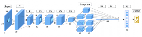
The design has eight layers: five convolutional and three completely connected. Max-pooling links the top 2 convolutional layers for maximum feature extraction. Each fully-connected layer connects directly to the third, fourth, and fifth convolutional layers [18]. The ReLu non-linear operational amplifier connects all convolutional layer outputs and fully-connected layer outputs. Figure 1 shows AlexNet architecture.
Figure 1. AlexNet architecture
Figure 2. VGGNet architecture
Figure 3. Google net architecture
The last softmax activation layer distributes the thousand class labels.
AlexNet gets a 256-by-256 RGB (3-channel) image. 60 million parameters, 650,000 neurons [19]. Dropout layers reduce overtraining. Dropped neurons don't propagate. These are the first two fully-connected layers.
2.2 VGGNet architecture
The first two layer’s employ 4096 channels, the third uses 1000 channels (one for each class) for ILSVRC classification, and the fourth uses softmax. All related levels follow this structure. ReLu activation functions are applied to hidden layers as the VGG network advances as shown in Figure 2.
2.3 GoogLeNet architecture
The GoogLeNet architecture is comprised of 27 pooling levels and has a total of 22 stacked layers [20]. In all, there are nine inception modules that are arranged in a linear fashion. The global average pooling layer is linked to the terminals of the inception modules. Figure 3 shows the whole of the GoogLeNet architecture at a reduced scale.
3.1 Dataset description
The dataset has two data tiers, making it unique among open-sourced solar forecasting datasets for deep learning studies.
3.2 Benchmark dataset
3 years' worth of reconstructed sky photos (6464) as well as simultaneous PV power production data at 1-min intervals, all of which are prepared for use in the construction of deep learning models.
3.3 Raw dataset
Overlapping high quality sky video footage (2048×2048) captured at 20 frames per second, sky picture frames (2048×2048), and historical PV power production data documented at 1-min frequency that fit different study objectives.
The data we collected at this website https://github.com/yuhao-nie/Stanford-solar-forecasting-dataset.
3.4 Pre-processing steps for image classification
To show how well-known pre-processing techniques affect basic convolutional networks' accuracy. Pre-processing processes follow.
Read image: We loaded picture-containing folders into arrays after putting the path to our image dataset in a variable to read the image.
Resize image: To illustrate the difference while resizing pictures, we'll develop two ways to display one and two images. We then create a processing mechanism that only accepts photographs.
Remove noise: Gaussian blurring removes noise. Animation programmes use it for picture clean up. Computer vision algorithms pre-process images using Gaussian smoothing to enhance visual structures at different sizes.
3.4.1 Image segmentation
In the given approach, a semi-automatic segmentation is used to transform a foggy image into a clear one depicting the sun. To achieve this, a pixel threshold needs to be set to judge and process the image. The determination of the pixel threshold depends on several factors and can be done using various techniques. Here are some common methods for determining the pixel threshold in image segmentation:
Image defogging
Image defogging using modified dark channel prior
For the purpose of transmission map estimation, a modified dark channel has been computed in this study. After that, the guided image filter is used to finish refining the transmission map (GIF). GIF is more effective than the other refinement filters since it shortens the total amount of time needed for calculation while refining the transmission map. As a result, the defogging process is improved. The proposed approach is used to calculate dark channel and atmospheric light from a foggy image. In order to estimate a transmission map which preserves gradient information, atmospheric light is used. The next step is to create a fog-free image using the revised transmission map.
3.4.2 Dark channel and atmospheric light estimation
Eq. (1) is used to calculate a dark channel in order to measure atmospheric light first. A filter of minimum window size ω is applied to compute dark channel, where ω is kept as 31×31.
$I_D=\min _{x \in w(k)}\left(\min _{y \in[R, G, B]} \quad I(y)\right)$ (1)
Dark channel is successfully calculated, and atmospheric light AL is estimated. Atmospheric light AL is a 3 by 1 vector with the greatest intensity values, and it is computed from 0.1% of the dark channel's brightest pixels.
3.4.3 Transmission map estimation and refinement
To calculate the transmission map, atmospheric light is employed. For each GB color channel, a transmission map according to Eq. (2) is calculated by dividing the input image by the corresponding color channel atmospheric light.
$T T(x)=1-\zeta\left[\frac{I(x)}{A}\right]$ (2)
In order to minimize oversaturation and entirely remove fog from the input image, the values of fFD1 and fFD2 are constant throughout the process and used to calculate fog density (FD).
The values of fFD1 and fFD2, which are 2.5 and 1 respectively, were obtained during cross-validation on the RESIDE dataset to evaluate the performance accuracy of a proposed model. It is mentioned that these values are set as fixed values in the current context. However, to determine the rationality of these fixed values, it is important to consider the context and purpose of the model, as well as the specific requirements of the RESIDE dataset.
Adjusting the values of fFD1 and fFD2 based on a figure suggests that there may be specific visual or performance considerations involved. Without the specific details of the figure or the model being used, it is challenging to provide a precise explanation of the rationality behind these fixed values. However, it is possible to discuss some general aspects that may guide the selection of fixed values in similar scenarios:
Domain Knowledge: The rationality of fixed values often depends on domain knowledge and prior research in the field. Understanding the characteristics of the RESIDE dataset, the nature of the model being used, and the relationships between fFD1, fFD2, and the model's performance can help determine suitable fixed values.
Model Validation: The cross-validation process conducted on the RESIDE dataset helps assess the model's performance accuracy. The selection of fixed values may be based on achieving the best performance results during this evaluation process.
Trade-offs and Generalization: Fixed values can be selected to strike a balance between model complexity and generalization. If fFD1 and fFD2 are too specific or fine-tuned to the RESIDE dataset, the model may over fit and fail to generalize well to other datasets or real-world scenarios. Setting fixed values that allow for reasonable performance on the RESIDE dataset while maintaining generalizability is crucial.
To maintain gradient information, the transmission map must be refined after being computed. The refining procedure in our suggested technique uses guided image filters (GIF), where the input picture itself serves as the guiding image and an edge-preserving and smoothing filter. GIF is quicker than other refining filters because to the defogging algorithm's total processing cost.
$T T_{r e f}(x)=a_k T T_k+b_k \quad \forall k \in W_k$ (3)
where, a and b are constant linear coefficients in Wk, and Trefis a linear transform of T in a window of size W. Figure 4 illustrates a transmission map and a revised transmission map, respectively.
Figure 4. Transmission map refinement (Foggy image; Refined transmission maps)
After the completion of the transmission map's refinement process, the defogged picture is rebuilt using:
$R(x)=\frac{I(x)-A}{T_{r e f}\;+\epsilon}+A$ (4)
where, $\in$ is a constant with an extremely low value that prevents division by zero. Gamma correction is also employed to enhance the overall brightness of the rebuilt picture at the conclusion of the defogging method.
3.4.4 Segmentation-based image defogging using modified dark channel prior
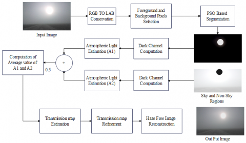
In this study, we have proposed an algorithm for defogging images by making use of image segmentation methodology. PSO-based segmentation techniques are used in order to complete the image segmentation process. Calculations are made for each segment's dark channel and atmospheric light. Using the average value of atmospheric light, transmission map estimates are made. The refining procedure is based on the guided image filter, as was mentioned in the preceding technique. To effectively remove fog particles, a segmentation-based method must provide high SSIM and PSNR values as well as a reduced MSE value. The proposed algorithm based on segmentation is shown in Figure 5.
In this approach, a semi-automatic segmentation is employed to transform a foggy image into a clear one depicting the sun. In order to transform an image into segments, the foreground and background pixels are each manually selected. Scribbles are drawn onto the image, which divides the image into background and foreground pixels and then PSO is applied for fast segmentation.
Figure 5. Segmentation-based image defogging using modified dark channel prior
Figure 6 displays the segmented pictures that were produced as a result. The dark channel for each segment is determined using the Eq. (5). While computing the dark channel, a filter with a minimum window size of ω is employed; for optimal results, the value of ω is maintained at 31 by 31 pixels throughout the process.
$\begin{aligned} & I_{D C P}\left(\operatorname{seg}_i\right)=\min \qquad\min I_{\operatorname{seg}\,_i}(Y) \\ & \qquad\qquad\quad x \in w(k) \quad y \in[R, G, B] \\ & \end{aligned}$ (5)
The defogged image is fed to the CNN classifier (AlexNet) to classify the image weather it is morning time production image, afternoon time production image, evening time production image. The performance of the proposed model is evaluated by using performance metric.
Figure 6. Image segmentation using PSO
(a) Foggy image, (b) Sky regions, (c) Non-sky regions
3.5 Performance metrics
The effectiveness of a technique is assessed in view of the confusion matrix's accuracy, sensitivity, precision, and F1-score.
Accuracy: It is the quantity of subjects that were effectively recognized out of all the subjects.
Accuracy $=\frac{T P+T N}{T P+T N+F P+F N}$ (6)
Sensitivity: The percentage of accurately positive labels that our computer recognises as being labels is called recall, also known as sensitivity.
Sensitivity $=\frac{T P}{T P+F N}$ (7)
Precision: By factoring in the overall number of precise predictions, it is feasible to determine the accuracy of an outlook. This idea also goes by the name of predictive value.
Precision $=\frac{T P}{T P+F P}$ (8)
F1-Score: The F1-score integrates precision and recall into a single score.
$F 1-$ score $=2 * \frac{\text {Precisison} * \text {Recall}}{\text {Precisison}+\text {Recall}}$ (9)
Specificity: The negative has been correctly categorized by the algorithm as specificity.
Specificity $=\frac{T N}{T N+F P}$ (10)
MATLAB 2020a is used to implement the model. Three sky test photos are analyzed. Analyzing the effect of the number of iterations on the results of model calculation involves understanding the concept of iterations in the specific context of the implemented model. Iterations typically refer to the number of times a certain operation or calculation is repeated within the model. It can be related to training iterations, optimization iterations, or any other specific operation that involves iterating over the data or model parameters.
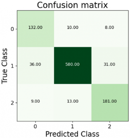
Figure 7. AlexNet
In this study, 1000 images are collected from the dataset. morning time production have 150 images, afternoon time production time have 647 images and evening time production have 203 images. The confusion matrix of the three architectures AlexNet, GoogLeNet, and VGGNet are given in below figures.
Figure 7 shows the confusion matrix of the AlexNet, it displays 3 classes in which 0 represents morning time production, 1 represents afternoon time production, and 2 represents evening time production. From the figure it is observable that the AlexNet classifies 132 morning time production images, and 580 afternoon time production images and 181 evening time production images. There are some misclassifications, 10 morning time production images are classified as afternoon time production images, 8 morning time production images are classified as evening time production images. 36 afternoon time production images are classified as morning time production images; 31 afternoon time production images are classified as evening time production images; 9 evening time production images are classified as morning time production image; 13 evening time production images are classified as afternoon time production images.
Figure 8. GoogLeNet
Figure 9. VGGNet
Figure 8 shows the confusion matrix of the GoogLeNet, it displays 3 classes in which 0 represents morning time production, 1 represents afternoon time production, and 2 represents evening time production. From the figure it is observable that the GoogLeNet classifies 131 morning time production images, and 540 afternoon time production images and 167 evening time production images. There are some misclassifications, 10 morning time production images are classified as afternoon time production images, 9 morning time production images are classified as evening time production images. 56 afternoon time production images are classified as morning time production images; 51 afternoon time production images are classified as evening time production images. 17 evening time production images are classified as morning time production image; 19 evening time production images are classified as afternoon time production images.
Figure 9 shows the confusion matrix of the VGGNet, it displays 3 classes in which 0 represents morning time production, 1 represents afternoon time production, and 2 represents evening time production. From the figure it is observable that the VGGNet classifies 126 morning time production images, and 521 afternoon time production images and 150 evening time production images. There are some misclassifications, 13 morning time production images are classified as afternoon time production images, 11 morning time production images are classified as evening time production images. 64 afternoon time production images are classified as morning time production images; 62 afternoon time production images are classified as evening time production images. 24 evening time production images are classified as morning time production image; 29 evening time production images are classified as afternoon time production images.
To evaluate the effectiveness of the architectures, the performance parameters are calculated such as Accuracy, Sensitivity, and Specificity and are visualized in Figure 10.
The average accuracy of AlexNet is 94.20%, GoogLeNet is 90.80%, and VGGNet is 88.40% in detecting the sun region. It suggests that AlexNet is the most accurate among the three models. Robustness refers to the ability of a model to maintain its performance across various conditions, including changes in input data, variations in the environment, and potential challenges. Figure 11 shows accuracy and loss of AlexNet.
Figure 10. Accuracy of architectures
To further discuss the robustness of the accuracy, it is important to analyze the model's performance in these different scenarios and evaluate its ability to maintain high accuracy. By examining data variability, generalization, outliers and anomalies, adversarial attacks, and transfer learning, we can gain a comprehensive understanding of the model's robustness in accurately detecting the sun region.
Figure 11. Accuracy and loss of AlexNet
Figure 12. Specificity of architectures
Figure 13. Sensitivity of architectures
The specificity of AlexNet architectures is 95.63%, GoogLeNet architectures is 91.41% and VGGNet architectures is 89.60% as shown in Figure 12. By this, it is observable that the sensitivity of the AlexNet architectures is high compared to GoogLeNet, and VGGNet.
Figure 13 shows that the sensitivity of AlexNet architectures is 89.27%, GoogLeNet architectures is 87.33% and VGGNet architectures is 81.82%. By this, it is observable that the sensitivity of the AlexNet architectures is high compared to GoogLeNet, and VGGNet.
The given sensitivity values (89.27% for AlexNet and 87.33% for GoogLeNet, VGGNet is 81.82%) indicate that the models are correctly identifying a high percentage of positive instances, but the sensitivity is still considered relatively low. Sensitivity, also known as the true positive rate, measures the proportion of actual positive instances that are correctly identified by the model. A relatively low sensitivity can be attributed to several factors such as insufficient training data, inadequate model complexity and imbalanced data. The comparison is shown in Table 1.
Table 1. Comparison of AlexNet parameters with other architectures
|
Architectures |
Accuracy (%) |
Specificity (%) |
Sensitivity (%) |
|
AlexNet |
94.20 |
95.63 |
89.27 |
|
GoogLeNet |
90.80 |
91.41 |
87.33 |
|
VGGNet |
88.40 |
89.60 |
81.82 |
In this study, we performed sky image classification based solar power prediction using CNN. For our experimental results MATLAB 2020a is used. In this work, our proposed model is AlexNet architecture of CNN. The PSO based segmentation method is used to defog the sun image and the defogged image is fed to the proposed CNN model. The performance metrics is used to evaluate the accuracy, specificity, sensitivity for each and every model. To know the accuracy of our proposed model, we compared the suggested AlexNet to the other two models (VGGNet, GoogLeNet) reveals that the proposed AlexNet has the best accuracy. The average accuracy of AlexNet architectures is 94.20%, GoogLeNet architectures is 90.80% and VGGNet architectures is 88.40%. By this, it is observable that the AlexNet architectures is more accurate in detecting the sun region.
We are thankful to the reviewers for their valuable comments and suggestions which helped us to improve the paper. We also thank our colleagues for their assistance in the preparation of this paper. Finally, we thank the computer science department at university for providing us with the necessary infrastructure and resources required to carry out this research.
[1] Pothineni, D., Oswald, M.R., Poland, J., Pollefeys, M. (2019). Kloudnet: Deep learning for sky image analysis and irradiance forecasting. In Pattern Recognition: 40th German Conference, GCPR 2018, Stuttgart, Germany, pp. 535-551. https://doi.org/10.1007/978-3-030-12939-2
[2] Xie, W., Liu, D., Yang, M., Chen, S., Wang, B., Wang, Z., Xia, Y.W., Liu, Y., Wang, Y.R., Zhang, C. (2020). SegCloud: A novel cloud image segmentation model using a deep convolutional neural network for ground-based all-sky-view camera observation. Atmospheric Measurement Techniques, 13(4): 1953-1961. https://doi.org/10.5194/amt-13-1953-2020
[3] Czarnecki, J.M.P., Samiappan, S., Zhou, M., McCraine, C.D., Wasson, L.L. (2021). Real-time automated classification of sky conditions using deep learning and edge computing. Remote Sensing, 13(19): 3859. https://doi.org/10.3390/rs13193859
[4] Fabel, Y., Nouri, B., Wilbert, S., et al. (2022). Applying self-supervised learning for semantic cloud segmentation of all-sky images. Atmospheric Measurement Techniques, 15(3): 797-809. https://doi.org/10.5194/amt-15-797-2022
[5] Wang, F., Xuan, Z., Zhen, Z., Li, Y., Li, K., Zhao, L., Shafie-khah, M., Catalão, J.P. (2020). A minutely solar irradiance forecasting method based on real-time sky image-irradiance mapping model. Energy Conversion and Management, 220: 113075. https://doi.org/10.1016/j.enconman.2020.113075
[6] Rajagukguk, R.A., Ramadhan, R.A., Lee, H.J. (2020). A review on deep learning models for forecasting time series data of solar irradiance and photovoltaic power. Energies, 13(24): 6623. https://doi.org/10.3390/en13246623
[7] Liu, Y., Li, H., Wang, M. (2017). Single image dehazing via large sky region segmentation and multiscale opening dark channel model. IEEE Access, 5: 8890-8903. https://doi.org/10.1109/ACCESS.2017.2710305
[8] Choi, M., Rachunok, B., Nateghi, R. (2021). Short-term solar irradiance forecasting using convolutional neural networks and cloud imagery. Environmental Research Letters, 16(4): 044045. https://doi.org/10.1088/1748-9326/abe06d
[9] Paletta, Q., Lasenby, J. (2020). Convolutional neural networks applied to sky images for short-term solar irradiance forecasting. arXiv preprint arXiv:2005.11246. http://arxiv.org/abs/2005.11246.
[10] Martins, V.S., Kaleita, A.L., Gelder, B.K., da Silveira, H. L., Abe, C.A. (2020). Exploring multiscale object-based convolutional neural network (multi-OCNN) for remote sensing image classification at high spatial resolution. ISPRS Journal of Photogrammetry and Remote Sensing, 168: 56-73. https://doi.org/10.1016/j.isprsjprs.2020.08.004
[11] Jiang, H., Gu, Y., Xie, Y., Yang, R., Zhang, Y. (2020). Solar irradiance capturing in cloudy sky days-a convolutional neural network based image regression approach. IEEE Access, 8: 22235-22248. https://doi.org/10.1109/ACCESS.2020.2969549
[12] Nie, Y., Paletta, Q., Scotta, A., et al. (2022). Sky-image-based solar forecasting using deep learning with multi-location data: Training models locally, globally or via transfer learning? arXiv preprint arXiv:2211.02108. http://arxiv.org/abs/2211.02108.
[13] Shi, C., Wang, C., Wang, Y., Xiao, B. (2017). Deep convolutional activations-based features for ground-based cloud classification. IEEE Geoscience and Remote Sensing Letters, 14(6): 816-820. https://doi.org/10.1109/LGRS.2017.2681658
[14] Lin, Y., Duan, D., Hong, X., Han, X., Cheng, X., Yang, L., Cui, S. (2019). Transfer learning on the feature extractions of sky images for solar power production. In 2019 IEEE Power & Energy Society General Meeting (PESGM) Atlanta, GA, USA, pp. 1-5. https://doi.org/10.1109/PESGM40551.2019.8973423
[15] Ye, L., Cao, Z., Xiao, Y., Yang, Z. (2019). Supervised fine-grained cloud detection and recognition in whole-sky images. IEEE Transactions on Geoscience and Remote Sensing, 57(10): 7972-7985. https://doi.org/10.1109/TGRS.2019.2917612
[16] Zhen, Z., Pang, S., Wang, F., et al. (2019). Pattern classification and PSO optimal weights based sky images cloud motion speed calculation method for solar PV power forecasting. IEEE Transactions on Industry Applications, 55(4): 3331-3342. https://doi.org/10.1109/TIA.2019.2904927
[17] Kong, W., Jia, Y., Dong, Z.Y., Meng, K., Chai, S. (2020). Hybrid approaches based on deep whole-sky-image learning to photovoltaic generation forecasting. Applied Energy, 280: 115875. https://doi.org/10.1016/j.apenergy.2020.115875
[18] Sudharshan, K., Naveen, C., Vishnuram, P., Krishna Rao Kasagani, D.V.S., Nastasi, B. (2022). Systematic review on impact of different irradiance forecasting techniques for solar energy prediction. Energies, 15(17): 6267. https://doi.org/10.3390/en15176267
[19] Lian, J., Liu, T., Zhou, Y. (2023). Aurora classification in all-sky images via CNN-Transformer. Universe, 9(5): 230. https://doi.org/10.3390/universe9050230
[20] Park, S., Kim, Y., Ferrier, N.J., Collis, S.M., Sankaran, R., Beckman, P.H. (2021). Prediction of solar irradiance and photovoltaic solar energy product based on cloud coverage estimation using machine learning methods. Atmosphere, 12(3): 395. https://doi.org/10.3390/atmos12030395