Turab Selçuk![]()
© 2023 IIETA. This article is published by IIETA and is licensed under the CC BY 4.0 license (http://creativecommons.org/licenses/by/4.0/).
OPEN ACCESS
The accessory spleen, a condition affecting a subset of the population, often presents diagnostic challenges due to its potential for being mistaken for a tumor or cyst. This underscores the importance of accurate identification of the accessory spleen. In this study, the development of a patch-based hybrid Convolutional Neural Network (CNN) model designed for the automatic detection of the accessory spleen is presented. The proposed model applies a five-step process in the detection of the accessory spleen, encompassing the extraction of the potential accessory spleen region, extraction of features from this region, selection of consistent and significant features, integration of these features, and their subsequent classification. Specialist physicians were responsible for the extraction of the region of interest. For feature extraction, four distinct CNN architectures were employed (AlexNet, Vgg16, MobileNet, Resnet50), and the feature vectors derived from these architectures were integrated. The Neighborhood Components Analysis (NCA) and ReliefF algorithms were utilized for the selection of the most representative features, which were subsequently classified using Support Vector Machines (SVM) and k-Nearest Neighbors (k-NN). The study revealed that the highest performance was achieved through the combination of SVM and ReliefF, yielding an accuracy of 93.87% (evaluated via 10-fold cross-validation). The findings suggest that the proposed model could offer valuable decision support for physicians in the preliminary identification of the accessory spleen during clinical evaluations of tumors and similar structures resembling the accessory spleen.
accessory spleen, hybrid CNN model, feature extraction
Accessory spleens, which are variously-sized secondary spleens that form during the embryological development within the womb, present a unique characteristic in contrast to the normal spleen tissue [1-4]. These entities, which develop differently from the conventional spleen, typically are smaller in size and can range from a few millimeters to several centimeters. On average, the diameter of an accessory spleen is considered to be approximately 1 cm [5-7].
The presence of accessory spleens, which can be singular or multiple, is an anatomical condition observed in approximately 10% to 30% of the human population [8-10]. A true encapsulated accessory spleen is comprised of smooth muscle and elastic tissue [5]. Commonly, these accessory spleens are located in the hilus, the region where arteries enter the normal spleen [10]. However, the location in which accessory spleens develop within the human body can be variable [9, 10].
Apart from the hilus, accessory spleens can potentially form in several other regions within the human body, such as the tail of the pancreas, the stomach wall, intestinal wall, gastrosplenic ligaments, omentum, mesentery, and in the pelvis in females or scrotum in males [7-10]. Accessory spleens typically remain in the human body for a lifetime, often without producing any clinical symptoms. Therefore, they are usually asymptomatic [9, 10]. A representative CT image demonstrating the presence of an accessory spleen is provided in Figure 1.
Figure 1. CT image of accessory spleen
1.1 Related works
When the literature is examined, in a study conducted by Adem Aktürk in 2013, some features of accessory spleens in the computed tomography images taken for the abdominal region of 1000 patients were examined. As a result, it was emphasized that the vascular vessels feeding the accessory spleen can be detected to a large extent in thin-section computed tomography and the diagnosis can be made that distinguishes it from other organ structures that can be confused with the accessory spleen [11]. In another study conducted by Linguru et al. [12] in 2013, the volume of the spleen was automatically determined by labeling 172 spleen images (45 images of normal spleen, 127 images of abnormal spleen) created by computed tomography. The obtained results were compared and analyzed in the light of previous studies. An accuracy rate of 95.2% was obtained [12]. In a study conducted by Onur Osman and other authors in 2016, automatic segmentation of the injured spleen was performed using morphological features of the normal spleen, computed tomography and abdominal images, and computer-aided diagnosis (CAD) method was proposed. The sensitivity of the proposed system in this study was reported to be approximately 96.42% [13]. It has been stated that this proposed method can provide a faster and more robust diagnosis than existing methods. In a study conducted by Teomete et al. [14] in 2018, performed a computer-assisted diagnosis (CAD) labeling study by using spleen morphological features to automatically detect traumatic abdominal pathologies. The system in this study was approximately 97.63%. It has given a sensitivity and it has been emphasized that all other traumatic abdominal pathologies can be detected more successfully and more effectively. Humpire-Mamani et al. [15] proposed a deep learning-based spleen volume detection study and performed volume determination with an accuracy of up to 92% using computed tomography images of 1100 patients.
1.2 Problem statement
If a clinical symptom occurs due to accessory spleen, accessory spleen should be removed with a surgical intervention [3-6, 10]. If the person's normal spleen has problems such as injury, cyst, or tumor, the normal spleen may need to be surgically removed [5, 6]. In this case, the accessory spleen can function like a normal spleen [10]. If the person's normal spleen is working more than it should, and in this case, if the spleen tissue needs to be surgically removed, accessory spleens should also be removed [5, 6]. Accessory spleens can be easily detected for radiological imaging due to their presence in fatty tissue [2], but the accessory spleen may appear larger in imaging methods because it is a highly bloody tissue [5]. In addition, accessory spleens are usually visualized with the help of computed tomography, and when noticed, they can be confused with cysts or tumors [2, 5]. In this case, it is very important to know the presence of accessory spleens and to detect them correctly in order to prevent an incorrect intervention when the person has a clinical symptom or a problem with the normal spleen [8-10]. Therefore, we propose a CNN-based hybrid model for automatic detection of accessory spleen to provide decision support to specialist physicians.
1.3 Contributions of our study
The contributions of the proposed system are summarized below.
A new hybrid CNN model was introduced.
A dataset of CT images containing accessory spleen was created.
A CNN-based system was created for the detection of accessory spleen.
Accessory spleen was detected automatically with high success in the study.
It has been shown that a hybrid model can be more successful by combining classical CNN models.
A decision support system was created for specialist doctors for the preliminary diagnosis of accessory spleen.
2.1 Dataset
In this study, the dataset was obtained from a total of 390 individuals, 172 with accessory spleens and 218 without accessory spleens. There are a total of 1550 CT images. Accessory spleen is present in 684 of these images and absent in 866 of them. The ages of individuals range from 20 to 85 years. 182 of them are women and 208 of them are men. Other information of individuals was not taken care of because it was unimportant. The performance of the study was tested with both ten-fold cross validation and hold out validation. For hold out validation, 310 images (20%) are reserved for testing and 1240 (80%) images are reserved for training. Statistical information about the data set is given in Table 1.
Table 1. Statistical information of the data set
|
|
No Accessory Spleen |
Accessory Spleen |
|
Number of Person |
218 |
172 |
|
Number of Image |
866 |
684 |
|
Age (Mean±SD) |
29.54±8.32 |
32.52±11.97 |
|
Gender (M) |
106 (48.62%) |
102 (59.3%) |
2.2 Methods
In this study, a CNN-based hybrid model for the detection of accessory spleen is proposed. A five-step process was followed in the study of the model. These steps are obtaining patch images of accessory spleen from the CT image, feature extraction, feature fusion feature selection and classification. In the first step, 16 patch images of 32×32 were obtained from 128×128 images created by the doctor from the roi regions. In the second step, patch images were fed to AlexNet [16], Vgg16 [17], ResNet50 [18], MobileNetV2 [19] CNN models to obtain features of patch images. Each model obtained a feature vector of 1×1000 for a patch image from the fully connected layer. For 16 patch images, a total of 16000 features were obtained from each model. In the third stage, a feature vector of 1×64000 was created by combining the feature vectors. In the fourth stage, feature selection based on NCA and ReliefF was made to extract the most decisive features in classification performance. These features selected in the last step were classified by SVM and k-NN. The schematic representation of the study is given in Figure 2 and the pseudo code is given in algorithm 1. Each of the process steps is described in detail in the following sections.
|
Algorithm 1. Pseudocode of the proposed patch-based model |
|
|
Input: Accessory Spleen Dataset (asd) |
|
|
Output: Classification Result |
|
|
00 |
Load asd |
|
01 |
for i=1 to N // N is the number of Images |
|
02 |
I=asdi // Read each image (I) from dataset |
|
03 |
Ir=roi(I) // Ir (256 x 256) is ROI of I |
|
04 |
Resize the Ir to 128 x 128 |
|
05 |
for k=1 to 16 |
|
06 |
Ip=Irk |
|
07 |
F1=AlexNet(Ip) // Extract to feature with AlexNet |
|
08 |
F2= Vgg16(Ip) // Extract to feature with Vgg16 |
|
09 |
F3=ResNet50(Ip) // Extract to feature with ResNet |
|
10 |
F4=MobileNet(Ip) // Extract to feature with MobiletNet |
|
11 |
F=merg (f1, f2, f3, f4) |
|
13 |
end for k |
|
14 |
end for i |
|
15 |
Normalize fT using min-max normalization |
|
16 |
$F_s=f n c a(F)$ or $F_s=f r l f(F)$ //Apply NCA and ReliefF to F |
|
17 |
Select the top 1000 features |
|
18 |
SVM(Fs,class) // Export selected features to the cubic SVM classifier. |
|
19 |
Obtain classification results with 10-fold CV and 80:20 hold-out validation |
Figure 2. Proposed hybrid model
Step 1: Obtaining patch images
In this section, firstly, redundant regions without AS were removed from the original CT images. The ROI image determined by the doctor was obtained as 256×256. These images have been resized to 128×128. Then, 16 patch images of 32×32 dimensions were created on these images.
Step 2: Feature extraction
Feature extraction is the most advantageous feature of traditional machine learning algorithms. The performance of deep learning networks is directly related to identifying features with high classification ability. Deep learning models provide high classification performance thanks to its multiple layers. However, this creates computational complexity. In order to reduce this complexity, pre-trained models (AlexNet, Vgg16, ResNet50, MobileNetV2) were used in this study. These 4 models have been chosen because they have high performance in classification problems. A feature vector of 1x1000 dimensions was obtained for each patch image from the fully connected layers of these models. Since each dimensioned accessory image consists of 16 patches, a total of 16000 features were obtained from each model. I is the patch number and Ipi is the ith patch image F1, F2, F3, F4 represent feature vectors of 16 patch images obtained with AlexNet, Vgg16, MobileNetV2 and ResNet50, respectively.
$F_1=\sum_{i=1}^{16} \operatorname{AlexNet}\left(I_{p_i}\right)$ (1)
$F_2=\sum_{i=1}^{16} V g g 16\left(I_{p_i}\right)$ (2)
$F_3=\sum_{i=1}^{16}$ MobileNetV2 $\left(I_{p_i}\right)$ (3)
$F_4=\sum_{i=1}^{16} \operatorname{ResNet50}\left(I_{p_i}\right)$ (4)
Step 3. Feature margining
Different network models extract different features from an image. The fact that the feature vector of the image contains different features directly affects the classification performance. For this purpose, feature fusion was used in the study. F1, F2, F3, F4 feature vectors from the fully connected layer of each model were combined as in Eq. (5) and a 1×64000 F feature vector of each accessory spleen image was obtained. Here U is the concatenation operator.
$F=F_1 \cup F_2 \cup F_3 \cup F_4$ (5)
Step 4: Feature selection
In classification problems, feature selection is used to obtain the most distinctive features in the feature vector. In addition, complex calculations and high processing time caused by unnecessary features are avoided. For this purpose, ReliefF [20] and Neighborhood component analysis NCA [21] feature selection algorithms were used to determine the most distinctive features from the 1×64000 feature vector and to create a subset of the feature vector.
Neighborhood component analysis (NCA): It assigns a coefficient to each feature. These coefficients are weighted according to the relationship between the features. Features with a high coefficient are enhanced, while features with a low coefficient are disabled. NCA is formulated as an optimization problem [20]. The feature selection process of NCA is explained below.
$F_s=f n c a(F)$ (6)
Here, F is the merged feature vector, fnca is the NCA function, and is the selected feature vector. Its mathematical expression is given in Eq. (7).
$\vec{w}=\arg _w \max \sum_{i=1}^n p_i-\lambda \sum_{r=1}^d w_r^2$ (7)
Here, $\vec{w}$ is the weight vector, pi is the probability of predicting the correct class of the classifier, wr is the weighting coefficient of the r'th feature, and λ is the correction coefficient. It improves the generalization coefficient of NCA. λ makes the weights of unimportant features zero. A large λ will reset the weighting coefficients of all features. That's why choosing the right value is important.
ReliefF: It is one of the distance-based feature selection algorithms [21]. It uses a Manhattan distance-based function. It is weighted depending on the distance value. Positive values highlight important features, while negative values suppress unimportant features (Eq. (8)).
$R l f_{\text {weight }}=R F(f, t)$ (8)
Here, Rlfweight represents weight values, RF weight function. F denotes the feature vector and t denotes the targeted values. The formula as in Eq. (9) is applied to remove the features with negative values.
$\begin{gathered}f^*(h)=\operatorname{feat}(k),\text { if } \operatorname{Rlf}_{\text {weight }}(k)>0, h=h+1, h \leq k, k=\{1,2,3 . .1000\}\end{gathered}$ (9)
Here, f*(h) represents features with positive value. The feature selection process of ReliefF is explained below.
$F_s=f r l f(F)$ (10)
Here, F is the merged feature vector, frlf is the ReliefF function, and Fs is the selected feature vector.
Step 5: Classification
The most distinctive 1000 feature vectors selected by ReliefF and NCA were given to the SVM and k-NN classifier. Ten-fold cross validation and hold out cross validation were used as classification strategy.
The proposed model was created in Matlab (2021b) environment. The computer used in the study has a 64-bit 2.30 GHz processor and 16 GB of RAM. Figure 1 shows the performance of the proposed model and pre-trained models (AlexNet, Vgg16, ResNet50, MobileNetV2) in accessory spleen detection. The parameters of the algorithms are given in Table 2. Confusion matrix was used to evaluate the performance of the proposed model. The confusion matrix offers a comprehensive assessment. Ten performance parameters were obtained from the confusion matrix. These parameters are accuracy (A), sensitivity (SN), specificity (SP), precision (P), F1 score (F1), misclassification rate (M), negative predictive value (NPV), false positive rate (FPR), false discovery. rate (FDR), false negative rate (FNR), and True positives (TP), true negatives (TN), false positives (FP), and false negatives (FN). The results obtained in Table 3 are presented in detail.
Table 2. Parameters of the algorithms
|
Phase |
Algorithm/Architecture |
Hyperparameter |
|
Feature Extraction |
AlexNet |
Total Parameters: 62 million Number of Layers: 25 Output: FC8 |
|
Vgg16 |
Total Parameters: 138 million Number of Layers: 41 Output: FC8 |
|
|
ResNet50 |
Total Parameters: Over 23 million Number of Layers: 50 Output: FC1000 |
|
|
MobileNetV2 |
Total Parameters: 3.4 million Number of Layers: 154 Output: logits |
|
|
Feature Selection |
NCA |
Solver: Stochastic Gradient Descent (SGD) Iteration: 10000 |
|
ReliefF |
Nearest neighbors Value (K): 2 Distance Scale Factor (Sigma): Infinitive |
|
|
Classification |
SVM |
Kernel: Cubic polinomial, Validation: Ten-Fold Kernel Scale: Auto |
|
k-NN |
Number of Neighbors: 2 Distance Metric: Euclidean |
Table 3. The obtained performance values
|
|
|
|
|
|
Proposed Model |
|
|
METRICS |
AlexNet |
Vgg16 |
ResNet50 |
MobileNet |
ReliefF |
NCA |
|
A(%) |
89.85 |
88.89 |
89.45 |
90.50 |
93.87 |
92.23 |
|
SN(%) |
90.82 |
89.8 |
89.80 |
90.91 |
94.16 |
92.86 |
|
SP(%) |
88.89 |
88. 00 |
89.11 |
90.10 |
93.59 |
91.61 |
|
P(%) |
89. 00 |
88. 00 |
88.89 |
90. 00 |
93. 55 |
91.67 |
|
F1(%) |
89.9 |
88.89 |
89.34 |
90.45 |
93.85 |
92.26 |
|
M(%) |
10.15 |
11.11 |
10.55 |
9.50 |
6.13 |
7.77 |
|
NPV(%) |
90.72 |
89.8 |
90. 00 |
91. 00 |
94. 19 |
92.81 |
|
FPR(%) |
11.11 |
12. 0 |
10.89 |
9.90 |
6.41 |
8.39 |
|
FDR(%) |
11. 00 |
12. 00 |
11.11 |
10. 00 |
6. 45 |
8. 33 |
|
FNR(%) |
9.18 |
10.20 |
10.20 |
9.09 |
6.84 |
7.14 |
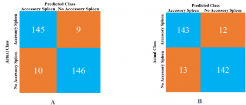
Figure 3. Confusion matrix obtained by SVM classifier and feature selection algorithms A. ReliefF B. NCA
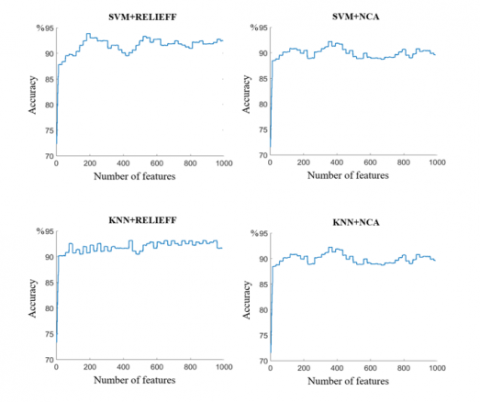
Figure 4. Change in accuracy values according to different classifier and feature selection algorithms
According to Table 3, the highest performance values among the pre-trained models were obtained with MobileNetV2 (Accuracy 90.5%, Sensitivity 90.9%, Specify 90.10%). ReliefF and NCA feature selection algorithms are used in the proposed hybrid model to increase the detection performance of AS. Using the features selected by ReliefF, 93.87% Accuracy, 94.16% Sensitivity and 93.59% Specificity were obtained in the detection of AS. 92.23% Accuracy, 92.86% Sensitivity and 91.61% Specificity were obtained in the detection of AS by using the selected feature with NCA. The performance of the study was tested with both ten-fold cross validation and hold out cross validation (19.3% test and 80.7% train). Different performance values were obtained by using different classifier and feature selection algorithms. The obtained values show that SVM has a higher performance of approximately 1% compared to k-NN. The highest performance was obtained with hold out CV and SVM+ReliefF as 93.87%. Table 3 summarizes the results obtained. Figure 3 shows the confusion matrices obtained using ReliefF and NCA. The highest performance SVM classifier and ReliefF feature selection algorithm were obtained. The 1000 features, which are the most determinant in the 1×64000 feature vector, are analyzed and their accuracy changes are given in Figure 4. As can be seen in Figure 4, when SVM+ReliefF algorithms are used together, the maximum accuracy value of 93.87% was obtained with the first 195 features. The lowest performance was obtained when the k-NN classifier and NCA feature selection algorithm were used together. The accuracy value obtained using the first 146 features was 91.85%.
The proposed model in the study is more successful than the classical and pre-trained models for the detection of accessory spleen. A classification is made with 1000 features from the fully connected layer of a pre-trained CNN model. The proposed model, on the other hand, was selected as the most distinctive 1000 features among 64000 features obtained from 4 different CNN models. In this way, a higher accuracy value was obtained with a hybrid model in which the best features selected by different models were used. A disorder that occurs during the shooting of some individuals negatively affects the performance of the proposed model. In some images, accessory spleen sizes were far below the average and could not be detected. This caused False Negatives to occur. All of the false negative images resulted from such a situation. Figure 5 shows sample images of false positives, false negatives, true positives, and true negatives.
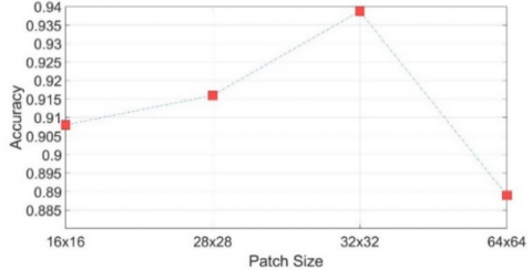
In medical images, especially CT images, the area of interest is usually in a small part of the image. Therefore, instead of analyzing the whole image, dividing the relevant region in the image into patches is necessary both in terms of performance and to reduce the processor load. In addition, the size of the selected patch image and its size to include the relevant lesion or tissue is an important criterion for success. The position of the accessory spleen in the CT image was determined by the specialist doctor. This area of interest covers a 128×128 region. As seen in Figure 5, the accessory spleen can be found in different locations within this area determined for each CT image in the data set. Accessory spleens in the dataset are of variable size, from approximately 20×20 to 30×30 pixels in the whole image. In this study, the effect of different patch sizes on performance was also investigated. For this purpose, patch images in 4 different (16×16, 28×28, 32×32, 64×64) sizes were used. In Figure 6, the accuracy values for the situation where SVM and ReliefF algorithms are used together for different patch sizes are given. The highest performance was obtained in 32×32 dimensions.
Figure 5. Example images showing different situations
Figure 6. Effect of patch sizes on detection performance
In this study, a patch-based hybrid CNN model was created for the detection of accessory spleen. This model includes four pre-trained models. The features from each model were combined. Then, the most decisive features were obtained with different feature selection algorithms. Accessory spleen was detected with k-NN and SVM classifiers. It has been observed that the proposed model is more successful in detecting the accessory spleen than other classical network models. With network models such as AlexNet, MobileNet, ResNet50, Vgg16, an average of 90.87% sensitivity, 89.50% specificity and 90.18% accuracy, respectively. In the proposed hybrid model, 94.16% sensitivity, 93.59% specificity and 93.87% accuracy were obtained. In the study, a local data set of abdominal CT images was created. In some cases, accessory spleen may show similar textural features with cancer tumors. In such cases, it is thought that the proposed system will guide expert radiologists in the detection of accessory spleen. In the next study, the data set will be updated by adding CT images containing tissues (tumor, cyst) that are similar to the accessory spleen. In this way, a new system will be developed that distinguishes the accessory spleen from other lesions.
I would like to thank Kamil Doğan, specialist in Radiology at Kahramanmaraş Sütçü İmam University Faculty of Medicine, for his contributions.
[1] Pforte, A. (2004). Epidemiology, diagnosis and therapy of pulmonary embolism. European Journal of Medical Research, 9: 171-179.
[2] Goldhaber, S.Z., Bounameaux, H. (2012). Pulmonary embolism and deep vein thrombosis. Lancet, 379(9828): 1835-1846. https://doi.org/10.1016/S0140-6736(11)61904-1
[3] Pena, E., Dennie, C. (2012). Acute and chronic pulmonary embolism: An in-depth review for radiologists through the use of frequently asked questions. Seminars in Ultrasound, CT and MRI, 33(6): 500-521. https://doi.org/10.1053/j.sult.2012.06.001
[4] Sadigh, G., Kelly, A.M., Cronin, P. (2011). Challenges, controversies, and hot topics in pulmonary embolism imaging. American Journal of Roentgenology, 196(3): 497-515. https://doi.org/10.2214/AJR.10.5830
[5] Kumamaru, K.K., Hunsaker, A.R., Kumamaru, H., George, E., Bedayat, A., Rybicki, F.J. (2013). Correlation between early direct communicationof positive CT pulmonary angiography findings and improved clinical outcomes. Chest, 144(5): 1546-1554. https://doi.org/10.1378/chest.13-0308
[6] Leung, A.N., Bull, T.M., Jaeschke, R., Lockwood, C.J., Boiselle, P.M., Hurwitz, L.M., James, A.H., McCullough, L.B., Menda, Y., Paidas, M.J., Royal, H.D., Tapson, V.F., Winer-Muram, H.T., Chervenak, F.A., Cody, D.D., McNitt-Gray, M.F., Stave, C.D., Tuttle, B.D. (2011). An Official American Thoracic Society/Society of Thoracic Radiology clinical practice guideline: evaluation of suspected pulmonary embolism in pregnancy. American Thoracic Society Documents, 184(10): 1200-1208. https://doi.org/10.1164/rccm.201108-1575ST
[7] Leung, A.N., Bull, T.M., Jaeschke, R., Lockwood, Ch.J., Boiselle, P.M., Hurwitz, L.M., James, A.H., McCullough, L.B., Menda, Y., Paidas, M.J., Royal, H.D., Tapson, V.F., Winer-Muram, H.T., Chervenak, F.A., Cody, D.D., McNitt-Gray, M.F., Stave, C.D., Tuttle, B.D. (2012). American thoracic society documents: An official American Thoracic Society / Society of Thoracic Radiology clinical practice guideline—evaluation of suspected pulmonary embolism in pregnancy. Radiology, 262(2): 635-646. https://doi.org/10.1148/radiol.11114045
[8] Konstantinides, S.V., Torbicki, A., Agnelli, G., et al. (2014). ESC guidelines on the diagnosis and management of acute pulmonary embolism. European Heart Journal, 35: 3033-3069.
[9] Hartmann, I.J.C., Prokop, M. (2002). Spiral CT in the diagnosis of acute pulmonary embolism. Medica Mundi, 46(3): 2-11.
[10] Stein, P., Fowler, S.E., Goodman, L.R., et al. (2006). Multidetector computed tomography for acute pulmonary embolism. The New England Journal of Medicine, 354(22): 2317-2327. https://doi.org/10.1056/NEJMoa052367
[11] Aktürk, A. (2013). Aksesuar Dalak Sıklığı ve Özelliklerinin Çok kesitli Bilgisayarlı Tomoğrafi ile Değerlendirilmesi, [Evaluation of the frequency and characteristics of accessory spleen with multislice computed tomography], Dicle University, 52p., Turkey, Available from: https://hdl.handle.net/11468/7362.
[12] Linguraru, M.G., Sandberg, J.K., Jones, E.C., Summers, R.M. (2013). Assessing splenomegaly: Automated volumetric analysis of the spleen. Academic Radiology, 20(6): 675-684. https://doi.org/10.1016/j.acra.2013.01.011
[13] Dandin, O., Teomete, U., Osman, O., Tulum, G., Ergin, T., Sabuncuoglu, M.Z. (2016). Automated segmentation of the injured spleen. International Journal of Computer Assisted Radiology and Surgery, 11: 351-368. https://doi.org/10.1007/s11548-015-1288-9
[14] Teomete, U., Tulum G, Ergin T., Cuce F., Koksal M., Dandin Ö., Osman O. (2018). Automated computer-aided diagnosis of splenic lesions due to abdominal trauma. Hippokratia, 22(2): 80-85
[15] Humpire-Mamani, G., Bukala, J., Scholten, E.T., Prokop, M., Van Ginneken, B., Jacobs, C. (2020). Fully Automatic Volume Measurement of the Spleen at CT Using Deep Learning. Radiology: Artificial Intelligence, 2(4). https://doi.org/10.1148/ryai.2020190102
[16] Krizhevsky, A., Sutskever, I., Hinton, G.E. (2017). Imagenet classification with deep convolutional neural networks. Communications of the ACM, 60(6): 84-90. https://doi.org/10.1145/3065386
[17] Simonyan, K., Zisserman, A. (2014). Very deep convolutional networks for large-scale image recognition. https://doi.org/10.48550/arXiv.1409.1556.
[18] He, K.M., Zhang, X.Y., Ren, S.Q., Sun, J. (2016). Deep residual learning for image recognition. Proceedings of the IEEE Conference on Computer Vision and Pattern Recognition, pp. 770-778. https://doi.org/10.1109/CVPR.2016.90
[19] Sandler, M., Howard, A., Zhu, M.L., Zhmoginov, A., Chen, L.C. (2018). Mobilenetv2: Inverted residuals and linear bottlenecks. In Proceedings of the IEEE Conference on Computer Vision and Pattern Recognition, pp. 4510-4520. https://doi.org/10.1109/CVPR.2018.00474
[20] Kira, K., Rendell, L.A. (1992). A practical approach to feature selection. Machine Learning Proceedings 1992, pp. 249-256. https://doi.org/10.1016/B978-1-55860-247-2.50037-1
[21] Yang, W., Wang, K.Q., Zuo, W.M. (2012). Neighborhood component feature selection for high-dimensional data. Journal of Computers, 7(1): 161-168. https://doi.org/10.4304/jcp.7.1.161-168