Gajula Srinivasarao![]() | Vullanki Rajesh
| Vullanki Rajesh![]() | Kayam Saikumar
| Kayam Saikumar![]() | Mohamed Baza*
| Mohamed Baza*![]() | Gautam Srivastava
| Gautam Srivastava![]() | Maazen Alsabaan
| Maazen Alsabaan![]()
© 2023 IIETA. This article is published by IIETA and is licensed under the CC BY 4.0 license (http://creativecommons.org/licenses/by/4.0/).
OPEN ACCESS
Early and accurate diagnosis of brain tumors is crucial in the medical field, as undetected or misdiagnosed tumors can lead to sudden death. Traditional models for diagnosing brain tumors suffer from low Time of Conversion (ToC) and low accuracy, contributing to a high mortality rate among the 5 million people affected by brain disease annually, as reported by the World Health Organization (WHO). Previous methods, such as Elastic Net Regression (ENR), Logistic Regression (LR), and other machine learning models, struggle to accurately locate and identify brain lesions. Moreover, these models are not suited for cloud-based platforms. To address this issue, we developed a sophisticated, cloud-based brain abnormality detection application using the LeNet-5 Convolutional Neural Network (CNN) on the DriveHQ platform. The pre-trained LeNet-5 model extracts features from ADNI-1, ADNI-2, and MIRIAD datasets. Real-time MRI brain images were collected from Manipal Hospital in Vijayawada, Andhra Pradesh, India. The LeNet-5 model employs hidden layers, flattened layers, max-pooling layers, dense layers, and ReLu layers for optimal performance. Our 2D-LeNet-5 CNN approach preprocesses images using split and merge techniques of binary mask segmentation. The Python 3.7 software tool was used to train and test datasets to identify abnormalities in MRI brain images. The proposed application achieved remarkable performance metrics, including 99.65% accuracy, 99.59% sensitivity, 99.72% F1-score, 99.25% recall, 59.32 PSNR, and 0.9929 MCC. These results demonstrate the superiority of our methodology in comparison to existing models, making it a promising solution for cloud-based brain tumor diagnosis and recognition.
MRI brain image, CNN, LeNet-5, cloud network, brain tumor, DriveHQ
The diagnosis of brain tumors and diseases constitutes a critical area of study in the field of medical applications. Brain tumors arise from abnormal cell structures in the human brain and can be classified as benign, malignant, or metastatic. Early and accurate diagnosis is crucial for saving lives, as brain diseases and tumors can grow rapidly and negatively affect the nervous system. The location and dimensions of tumors play a significant role in determining the appropriate treatment for patients. Treatment of brain diseases largely depends on the type, size, and location of the tumor. According to the American Brain Cancer Institute, approximately 5 million individuals are affected by brain tumors and anomalies annually, with 1 million succumbing to these disorders. Magnetic resonance imaging (MRI) preprocessing and deep learning can aid in the medical diagnosis process, focusing on the efficient detection of tumors or cancerous cells in healthy tissues. This approach can assist with early-stage disease detection, identification of the affected area percentage, and tumor dimensions. Lim and Mandava [1] extensively discussed tumor-affected regions and area dimensions, employing a simple manual segmentation process. ResNet architecture using convolutional neural networks (CNN) can be employed for real-time MRI image segmentation and classification, as described in study [2]. Image preprocessing and contrast adjustment using MRI brain data were explored by Zhu et al. [3].
Medical scan images, including MRI, are a critical component of diagnosing deep infections in human organs through a layered methodology diagnosis process. This technique provides both medical and technical information, as various models have been investigated with different technologies [4]. Among the available medical diagnosis models, MRI is an effective radiation modality that offers crucial information regarding tumor location, size, and classification. It identifies the nature of protons based on radio frequency and equilibrium states [5]. MRI brain images contain extensive information related to the disease-affected area and the proportion of tumor content.
This research paper is structured as follows: Section 1 serves as an introduction to MRI brain abnormalities and the diagnosis process. Section 2 reviews recent advancements in brain tumor detection models. The implementation and simulation processes of the proposed deep learning model are detailed in Section 3. Section 4 presents the results and discussion of the suggested approach. The conclusion of the proposed brain tumor detection model is provided in Section 5. Lastly, Section 6 offers information on the dataset and data availability.
1.1 Appendix
World Health Organizations (WHO), Machine learning (ML), Convolution Neural Network (CNN), Magnetic Resonance Imaging (MRI), time of conversion (ToC), Area Under Curve (AUC).
The MRI scan images provide valuable data with a very high-resolution value which can quickly diagnose brain tissues such as blood oxygenation and water diffusion. The MRI scan images computationally differentiate the soft tissues with high diagnostic values and the sensitive tissues' density change values [6]. The most common degenerative brain illnesses are brain tumors, transient ischemic attack (TIA), and cancer, which afflict 60 million individuals worldwide [7]. Because of brain tumors Brain disorders like Transient ischemic attack impact almost 15% of the global populations [8]. Based on the clinical history, a diagnosis of Brain tumor brain disorders (ABD) occurs in 12 per 1000 people each year. The worldwide voice on Alzheimer's study includes a poll on various datasets, including essential sciences for cancers and brain diseases [9]. The miss-folding of brain MRI images is a feature of multi-modal methods for brain diseases. Various brain diseases impact millions of people worldwide, and biomarkers fluid method and neuro-image techniques may aid in identifying brain cancers and tumors [10]. The imported psychosis functionality identifies the cognitive relationships between brain abnormality disorders. By categorizing actual data with accessible datasets, deep learning systems could readily identify brain cancers and tumors [11]. When brain tumors and brain diseases obstruct human health circumstances, social activities and developments are no longer possible. Deep learning concepts are essential in future image processing applications. Many architectures like CNN, FCNN, and AlxNetwere failed to obtain information from hidden samples. Therefore, an advanced CNN, nothing but LeNet-5, is imported to overcome the above limitations.
The preceding section shows they may introduce different diseases to identify brain disorders. Reducing the MSE & false positive rate-FPR in identifying brain illnesses utilizing the rank confusion matrices approach proposed in study [12]. Various screening devices and apps may add to diagnosing individuals with brain disorders by identifying tumors [13]. Pattern recognition uses to characterize the early road map approach depending on the natural marking concept; this may assist in identifying the disorders in the patients’ brains who are experiencing unusual circumstances [14].
All the above models and ENR focus on and review different research projects and their study findings. Many models achieve excellent accuracy, throughput, and recall in this way. However, adjustments and improvements are required. Machine learning algorithms were employed in this study to identify diseases using threshold segmentation and logistic regression [15].
It is possible to analyze the Magnetic resonance imaging-MRI images to the ADNI-1, ADNI-2, & MIRIAD databases in real-time by exporting a database in the background. The first step introduces the image acquisition method to process MRI brain pictures. This methodology used three approaches to arrive at the concepts: image intensity modification, histogram equalization, and segmentation. The photo has been improved with varying values of pixel to new ranges for intensity modification [16]. Here, 0–255, 0–511, 0–1024, etc. are all valid values for the intensity axis. Those values are independent of the greyscale's low-to-high contrast range. It was modified to meet picture quality promises. The available MRI brain image-based disease classification models cannot get hidden sample information, but the architecture is easy to access. Functional MRI (fMRI) data preprocessing includes several techniques to clean and standardize data before statistical analysis. In most cases, researchers design ad hoc preprocessing processes for each new dataset, i.e., drawing on a broad toolkit. With significant breakthroughs in capture and processing, the complexity of these operations has been overwhelmed. The ability to automatically segment separating MRI brain pictures into white matter-WM, grey matter-GM, & cerebrospinal fluid-CSF are difficult for scientific study. Clinical diagnostics that aim better to understand the brain anatomy and function [17]. Here, they illustrated an MRI brain image segmentation methodology based on multiresolution edge detection, area selection, and methods for spatial & intensity cutoffs [18].
Using these segmentation structures, we may extract a region-of-interest-ROI image of the designs. The ROI is then adjusted using an automated threshold approach and threshold selection criteria. Segmentation examples of magnetic resonance imaging (MRI) brain scan at T1 & T2 weights, highlight the subtler characteristics of brain tissue [19]. It is the goal of a feature selection strategy, such as the class labels in classification, to pick a limited group of characteristics that minimizes duplication and increases the relevance to the objective. As a result, the machine learning model has a concise structure with a high degree of predicted accuracy based on the chosen essential attributes. Machine learning and knowledge discovery depend heavily on feature selection [20]. The (Support Vector Machine) SVM, Genetic algorithm (GA), (Random Forest Optimization) RFO and Decision Tree (DT) are facing more limitation like accuracy and ToC issues. This section has clearly defined brain diagnosis models and their limitations.
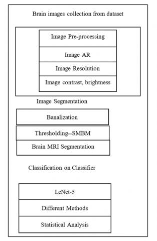
This section explains brain tumor lesion finding application with the LeNet-5 CNNdeep learning technique. The feature extraction, as well as the classification, have been performed to Auto stack CNN. The Split-and-Merge Binary Mask Threshold segmentation (SMBM) is employed as image enhancement to extract the object information. All of the MRI brain images used in the ANDI-1, ANDI-2, & MIRIAD datasets were publicly available online. Which is very suitable for the potential training process [21].
Figure 1. LeNet-5 architecture
The above Figure 1 clearly illustrates LeNet-5 MRI brain tumor detection. Within this approach, we use the Split-and-Merge binary masks segmentation method on sizable brain MRI picture collections for training purposes [22]. Once they have recovered all form & text characteristics, the SMBM segmentations can utilize as a potential objection’s detection phase. Image enhancement and segmentation steps can easily track the tumor or disease on brain radiology images. The auto stack training process extracts the features, where 14 classes are identified and employed in the CNN deep learning technique. The auto stack is nothing but layered architecture in parallel model to get statistical information related to brain. The classes are listed as 1 id: patient identification number 2 ccf: social security number (I replaced this with a dummy value of 0) 3 age: age in years 4 sex: sex (1 = male; 0 = female) 5 painloc: chest pain location (1 = substernal; 0 = otherwise) 6 painexer (1 = provoked by exertion; 0 = otherwise) 7 relrest (1 = relieved after rest; 0 = otherwise) 8 pncaden (sum of 5, 6, and 7) 9 cp: chest pain type -- Value 1: typical angina -- Value 2: atypical angina -- Value 3: non-anginal pain -- Value 4: asymptomatic 10 trestbps: resting blood pressure (in mm Hg on admission to the hospital) 11 htn 12 chol: serum cholestoral in mg/dl 13 smoke: I believe this is 1 = yes; 0 = no (is or is not a smoker) 14 cigs (cigarettes per day). The classification technique is applied to identify the original disease location and affected area in mm by the Dice score mechanism. The complete flow of the CNN technique can provide an MRI brain tumor location and size of the affected lesion. The split and merge binary mask segmentation can import mean standard deviation and variance parameters. They can find the statical analysis behind the deep learning model smooth Area under Curve (AUC). The mathematical computations for brain lesion extraction can be exact with LeNet-5. They can directly take the training from ANDI-1, ANDI-2, and MIRIAD datasets in .CSV format.
3.1 Brain MRI image enhancement
The input brain MRI images has been enhanced with histogram equalization techniques. The brain image's resolution, intensity, and brightness can be updated automatically to the histogram tool with python software. The supplied image's grayscale power remains between 80 and 250 dots per inch. Essential characteristics, including image contrast, Aspect Ratio-AR, resolution, & brightness, were supplied in stealth mode [23]. Adaptive histogram equalization is a process to extract edge-level features from an input image. The mapping can be applied to enhanced brain MRI images to load shape and text features. The histogram equalization can improve the picture's aspect ratio by matching the resolution.
$\begin{gathered}\text { pout }=\text { CV2.imread }\left({ }^{\prime} \text { pout.tif } \text { if }^{\prime}\right) ; \\ \text { pout }_{\text {imadjust }}=\text { CV2.imadjust }(\text { pout }) \\ \text { pout_histeq }=\text { CV2histeq }(\text { pout }) \\ \text { pout }_{\text {adapthisteq }}=\text { adapthisteq }(\text { pout })\end{gathered}$ (1)
The above Eq. (1) briefly explain tuning and pre-processing computations according to noise amplification as presented in the image. In some cases, image adjustment techniques drastically negatively affect the histogram properties; as a result, image perception is not up to the mark. Therefore, before applying segmentation and classification, there is a need to train the image with histogram enhancement.
The collected dataset has MRI brain images and the corresponding. CSV file text features data. The file consists of 14 classes: age, sex, frontal_lobe_1, frontal_lobe_2, frontal_lobe_3, medula_level_1_1, medula_level_1_2, medula_level_2_1, medula_level_2_2, medula_level_3_1, medula_level_3_2, optus_lobe_1, optus_lobe_2, and optus_lobe_3. The prototype application tests the LeNet-5 deep learning classifier on the cloud platform. The input dataset consists of 1lakh brain samples, where models like healthy, cancer, tumor, and various disease brain variants representation. The following example is trained using the CNN deep learning process to extract the features. The dataset has been normalized with statistical values from 0 to 1 for better correlation purposes such that it can get balanced from unstructured data conditions.
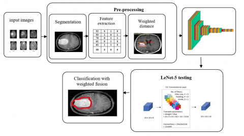
The above algorithm pre-processes mathematical steps related to MRI brain images. This pseudo-code and suitable packages have been implemented on the python 3.7.0 software tool. After this pre-processing, the idea was sent to feature extraction and classification stages, as shown in Figure 2, and the algorithm.
Figure 2. Brain disease diagnosis process
|
Algorithm for Normalizing MR Image Histograms |
|
Histogram of Function (X, Y) Input: MRI brain image input in 2 dimensions with positive integers for x and y. Output: high-quality image processing prior to picture capture. Whenever Y=0, Input Image = CV2.imread(pout); To Get Back (q, r) == (1, x) else Set (q, r) = CV2.imadjust (output image) In the event that X has worse pixel quality Answer = (Res+1) Using the formula: pout histeq = CV2histeq (output image) poutadapthisteq adapthisteq in the console, the resulting string will look like this: (final pre-processed image) End Res=r+1 then R=r-y, q=q+1; End End End histogram |
In this step histogram equalization process collects the input images from available dataset. To apply the local minima concept for pre-processing via transformation to adjust the dynamic gray pixel concept. After local minima divide the histogram local minima with specific gray level. Each partition of histogram has been trained to equalization process explained in Eqs. (2)-(4).
$\begin{aligned} & P_s(S)=P_r(r)\left|\frac{d_s}{d_r}\right| = & P_r(r)\left|\frac{1}{(L-1) P_r(r)}\right| = & \frac{1}{(L-1)} ; 0 \leq L-1\end{aligned}$ (2)
$\begin{gathered}\frac{d_s}{d_r}=\frac{d}{d_r} T(r) =\frac{d}{d_r}(L-1) \int_0^r P_r(w) d w =(L-1) P_r(r)\end{gathered}$ (3)
$s=T(r)=(L-1) \int_0^r P_r(w) d w$ (4)
Figure 3. Histogram equalizations
Figure 3 explains the histogram balancing and unbalancing of brain MRI pictures. The MRI images with the histogram process are perceptually good compared to the without-histogram image. The scale varies from 0 to 1600 DPI (history-done) and 0 to 900 DPI (without history). The pre-trained pictures are sent for image segmentation using the SMBM threshold method.
3.2 Segmentation
Here, we apply the procedure of split & merge binary mask threshold segmentations to an MRI of the brain to locate malignant tumors, anomalies, and individual cancer cells. SMBM thresholding is an essential imported image improvement technology to segment medical images correctly. Images might randomly slice into four equal parts, with each quarter representing a different but visually equal part of the image. Equal slices are successively merged to create segmented output for tumor detection. The parent and child structure with the quad tree model performs the SM segmentation process. In the SM process, they should apply homogeneity criteria on split regions. The splitting mechanism can make slices of equal size in all areas and calculate homogeneous regions continuously. Homogeneity in the area merges with the neighbor slices. Otherwise, the pieces are not merged. This mechanism has been repeated until all region images undergo the SM test. There should be a split test inhomogeneity to ascertain whether each separated region needs further splitting. The homogeneity principle depends on grey scale levels along with their thresholding. The threshold value can be determined using the local and global mean concepts [24]. The local mean is a particular grey-scale variance mechanism and the global mean is the complete image grey-scale variance. Both local mean and global means are segmentation concepts at threshold value selection; the local mean only suitable for RGB and Grayscale images with low noise level conditions. Considering the high noise level, the global mean concept is mandatory to trace out the threshold value. In this condition, they can decide the disease-affected pixels with abnormal locations in the brain.
$\sigma^2=(1 /(N-1)) \sum_{(r, c) \in R}[I(r, c)-\bar{I}]^2$ (5)
The Eq. (5) explains the variance calculation process using intensity computation.
$\bar{I}=(1 / N) \sum_{(r, c) \in \text { Region }} I(r, c)$ (6)
Eq. (6) describes the intensity calculations of selected images via the split and merge concept; here, R and C represent row and column, similarly, where N is the total amount of pixels in the area, as shown in Figure 4.
Figure 4. SM segmentation
$I_{\text {Mask }}(x, y)= \begin{cases}1 & \text { if } f_w^{\lambda_{\text {Gray }}}(x, y)>T \\ 0 & \text { if } f_{w \text { }}^{\lambda_{\text {Gray }}}(x, y) \leq T\end{cases}$ (7)
Figure 5. SM tree model
Figure 5 clearly explains the splitting process using the homogeneity principle. The brief explanation about the SM tree is something other than quadrant tree architecture. Eq. (7) provides information about binary masking from the image. T is the threshold value, and x and y define the threshold point coordinates.
The all-grey level values >T are treated as white pixel values (1), otherwise taken as black values (0). If this process continues, ones and zeros automatically change according to the interested area. The SM tree is a vital 125 branches quadrant model. In this, all sub-samples can process via the mask homogeneity principle. The mask provides split and merge instructions to the SM tree; as a result, grey-level pixels differentiate between zero and one. For example, if the tree's numerical value is greater than the sub-branch, it is considered zero; otherwise, one is taken into account [25].
$T=\max \left(\sigma^2\right)$ (8)
$A_{\text {mask }}=\sum_{x, y} I_{\text {Mask }}(x, y)$, for $I_{\text {Mask }}>0$ (9)
Eq. (8) is the maximum variance between the object and background. A mask is calculated as the total area of a binary mask among regions of interest, as shown in Eq. (9). This is an example of intensity calculation $I_w^{\lambda_c}(x, y)=f_w^{\lambda_c}(x, y) * I_{\text {Mask }}(x, y)$. The intensity matrix values can obtain through the convolution of the binary and intensity mask functions. Any sub-images with info larger than or equal to one-third of the sub-total image's size are chosen. $A_{\text {Mask }_j} \geq \frac{1}{3}\left[I_{\text {Mask }_j}(x, y)\right]$.
Figure 6. SMBM segmented image
Figure 6 clearly explains the Split and merge segmentation process. Here, they may quickly isolate aberrant or corrupted photos. The binary mask and split & merge process are more accurate in segmentation to extract information from the MRI brain images. The Split and merge binary mask segmentation process is applied on selected MRI brain images; using this concept of SMBM, all background and foreground samples are to be differentiated and get traced out by color labelling.
3.3 Extracting features
Using the LeNet-5, each sample has been extracted with described features to .csv file. Auto-stack technique is used extract micro features and loaded to available dataset. To obtain 14 features such as auto correlation (AC), contrast (C), correlation (CO), entropy (E), energy (EN), homogeneity (H), dissimilarity (D), sum of square variance (SSV), cluster shade (CS), cluster prominence (CP), inverse difference normalization (IDN), sum average predictor (SAP). LeNet-5 Auto-stack process is a third-order statistical model applied to generate MRI brain text features from grey-level pixels. The following text features have been collected using reference pixels according to the nine opposite pixel offset theory. θ = (45,45), (0,45), (315,45), (45,0), (0,0), (315,0), (45,315), (0,315), (315,315).
Figure 7. Auto-stack process on features
Figure 7 explains about co-occurrence between reference and original pixels. The left and right images provide information about the 9 pixels depicted opposite. The auto stack encoding process is reliable for moving the selected input image into different deep leaning layers like flatten layer, dense layer, max-pooling layer, and ReLU layer. The following layers provide information to LeNet-6 architecture where step-by-step pixel refining cloud performs simultaneously, and the brain abnormality pixels are classified.
$P(i, j)_{\left(\theta_1, \theta_2\right)}=\frac{1}{256^2} \sum_{x=1}^{512} \sum_{y=1}^{256}\left\{\begin{array}{c}0, \quad \text { if } L(x, y) \\ i \text { and } R(x+\Delta x, y+\Delta y)=j \\ 1, \text { otherwise }\end{array}\right.$ (10)
Eq. (10) explains the co-occurrence matrix resultant, where L stands for the left image & R for the right image. The rules below describe how the directions of matrices affect the x & y coordinates. The current technology for brain tumor detection is most prominent in operation, but they cannot identify an efficient and accurate diagnosis of the brain through this. The existing deep learning technologies like CNN, FCNN, ResNet, and AlexNet are limited in their architecture, and hidden layers cannot be identified as affected samples. The MRI brain images are processed through LeNet-5 architecture with 165 layers. The following framework hypothetically visualizes and obtains brain information to identify the affected area and the location.
if $\theta 1=0$ and $\theta 2=0$ then $\Delta x=0$ and $\Delta y=0$,
if $\theta 1=0$ and $\theta 2=45$ then $\Delta x=-1$ and $\Delta y=0$,
if $\theta 1=0$ and $\theta 2=315$ then $\Delta x=1$ and $\Delta y=0$,
if $\theta 1=45$ and $\theta 2=0$ then $\Delta x=0$ and $\Delta y=1$,
if $\theta 1=315$ and $\theta 2=0$ then $\Delta x=0$ and $\Delta y=-1$,
if $\theta 1=45$ and $\theta 2=45$ then $\Delta x=-1$ and $\Delta y=+1$,
if $\theta 1=315$ and $\theta 2=45$ then $\Delta x=-1$ and $\Delta y=-1$,
if $\theta 1=315$ and $\theta 2=45$ then $\Delta x=-1$ and $\Delta y=-1$,
if $\theta 1=315$ and $\theta 2=315$ then $\Delta x=1$ and $\Delta y=-1$,
if $\theta 1=45$ and $\theta 2=315$ then $\Delta x=1$ and $\Delta y=1$.
The resultant of the 9-pixel theory provides co-occurrence matrix information; if it is symmetric around the diagonal, then the scanned brain is healthy, and if it is asymmetrical, then the scanned brain is in an abnormal condition. Finally, 12 co-occurrence text features are extracted by the co-occurrence matrix. In addition, weighted mean and weighted distance features are implemented for estimating the disease size. The weighted mean is a parameter applied to identify irregularity of MRI brain image tumor based on the nearest distance between the diagonal co-occurrence matrix and the weighted mean. This parameter is high when there is a tumor in the MRI brain and low when the MRI brain image is standard in the stage. The 9-pixel theory can effectively provide a 1280×720 resolution image. With this clear picture, brain disease can be verified using five dark lines. They are continually varying their angle nine times per 1 resolution, so this concept, named as 9-pixel theory.
3.4 Input brain images
They utilized the Alzheimer's disease Neuroimaging Initiative (ADNI-1, ADNI-2) and MIRIAD Database to gather data for this research, as shown in Figure 8. The Eqs. (11)-(15) provide information about weighted mean co-occurrence where weighted mean is defined as Weighted mean (A, B) = |y-x| sin 45°.
$x=\frac{1}{256^2} \sum_{i=1}^{256} \sum_{j=1}^{256} i \cdot P(i, j)$ (11)
$y=\frac{1}{256^2} \sum_{i=1}^{256} \sum_{j=1}^{256} j \cdot P(i, j)$ (12)
$\begin{gathered}\text { Weighted mean }(A, B)=|y-x| \sin 45° \\ \text { uptrag }=\sum_i \sum_j d_{i j .} p(i, j)\end{gathered}$ (13)
lowtrag $=\sum_i \sum_j d_{i j .} p(i, j)$ (14)
Weighted distance $=\mid$ uptrag - lowtrag $\mid$ (15)
Table 1. Data set information
|
S No |
Name of Data Set |
Sample Size |
|
1 |
ANDI-1 |
1 lakh samples (open source) |
|
2 |
ANDI-2 |
1 lakh samples (open source) |
|
3 |
MIRIAD |
1 lakh samples (open source) |
CNN is a simple deep learning process, while many advancements still need to be included in addition to the limitations. An improved, reliable and competent model requires in upcoming architectures. Therefore 165 layered LeNet-5 model is implemented to overcome the limitations of CNN, as shown in Table 1.
Figure 8. Training set of MRI brain images
Figure 9. Tumor infected area and location estimation
The above analysis explains disease affected area, using the Euclidian distance principle, estimating the affected area in mm. The angle of tilting and variations have been providing 360° observations, such that diseases affected area is accessible to locate.
$\theta=\tan ^{-1} \frac{V_2}{V_1}$ (16)
Eq. (16) explains the angle calculation mathematical formula. It is applied to estimate the diseased area. The above MRI brain image has a brain tumor evaluated through the weighted distance theory. The continuous process of weighted mean, as well as weighted distance concepts, provides disease location and disease area, as shown in Figure 9. The following boundary analysis with left, right, top and bottom based location estimation providing exact abnormality detection with affected area.
3.5 Classification
In this section, brain image CNN classification performs using the LeNet-5 deep learning technique. When the extracted features are fed into a deep learning model, the resulting text features are utilized as a basis for further training. Diseases were classified & accurate information is provided through the usage of convolution layers, Max pooling layers, thick layers, flattened layers, & completely convolution layers. There are 7 stages to the activation’s functions used by LeNet-5. This layer’s compositions consists of 3 convolutional layers, two subsampling layers, & two fully linked layers. The input data design for the accept 32×32 pictures, which are the dimensions of the images sent to the following layer. Researchers such as Yann LeCun introduced the updated LeNet.
|
CNN: Mathematical Computations |
|
CNN functional classification Input: MRI brain image features Output: tumor location and affected area If input image features== (6×32×32) Feature maps== convolutions (6×32×32) $H_l=\operatorname{cover}\left(b_l * f_l\left(H_{l-1}\right)+i d\left(H_{l-1}\right)\right) ;$ Hl=input feature; else covert image size = cover(6×32×32); while S>0; subsampling (input image features); input images $\rightarrow$ sub images $\quad\left(H_F^*:=\right.$ $\operatorname{argminL} (X, Y, f)$ subfeatures to $f \in F)$; if N features == verified apply LeNet CNN on structured data $h_n=$ Fuc layers $\left(W_1 x_n+b_1\right)$ if L>0; Location $\hat{x}_n=g\left(W_2 h_n+b_2\right)$ else adjust (h, b); if A>0; affected area $\emptyset(\theta)=\underset{\theta, \theta^1}{\operatorname{argmin}} \frac{1}{n} \sum_{i=1}^n L\left(x^i, \hat{x}^i\right)$ else return to L; end if end if end while end if |
To process massive volumes of information, convolutional neural networks-CNN use feed-forward neural networks-NN with artificial neurons-AN that can respond to some of the cells in the coverage area. Based on the available dataset, LeNet-5 works to identify brain diagnosis checks. In the earlier research, they could recognize fully linked and activation layers in neural networks. But Convolutional and pooling layers are added in LeNet-5. All other ConvNets are part of LeNet-5. In the deep learning model, its simplest common activation functions seem to be Rectified Linear Unit-ReLu. A return value of 0 is generated for every negative input-I/p, whereas a return value of 1 is generated for all positive input-i/p values x. However, the ReLU function performs well in the vast majority of data voting, frequently utilized for hidden data extraction.
3.6 Data availability
The MRI brain image dataset collects from various organizations like ANDI in this research. After pre-processing the Images, data convert into CSV files; more of these samples trains through the LeNet-5 deep learning model.
3.7 Detection of brain tumors
Right here, the Brain tumor detection process explains through LeNet-5 Deep Learning (DL) approach. The LeNet-5 is a 7-layered architecture: these 3-convolutional layers present 2-sub sampling layers and 2-fully connected layers. The 2D- features like 32, 28, and 28 extracts the information in deep analysis. The following layers adjust the intensity that ranges from -0.1 to 1.1775 on grayscale shown in Figure 10.
Figure 10. Brain tumor detection DL process
Table 2. LeNet-5-layers
|
Model 1. “Sequential_1” LeNet -5 |
||
|
Layer (Type) |
Output Shape |
Parameters |
|
Conv2d_1 (conv2d) |
(None. 126, 126, 32) |
320 |
|
Max_pooling2d_1 (Max Pooling2) |
(None. 63, 63, 32) |
0 |
|
Conv2d_2 (conv2d) |
(None. 61, 61, 32) |
9248 |
|
Max_pooling2d_2 (Max Pooling2) |
(None. 30, 30, 32) |
0 |
|
Flatten_1 (Flatten) |
(None, 28800) |
0 |
|
Dense_1 (Dense) |
(None, 128) |
3686528 |
|
Dense_2 (Dense) |
(None, 2) |
258 |
|
Total params: 3,696,354 Trainable: 3,696,354 Non-trainable params:0 |
||
The standard deviation (SD), mean, and variance computations provide information about the classification. The trainable parameters (weight + bias) classify the disease location with color tracking. Convolutional and subsampling layers are also the two most crucial layer that constructs the LeNet-5, as shown in Table 2.
For this application, python, software3.7 version, and effective packages imports, the following application is run on Windows or any other OS with 8GB RAM through the DriveHQ cloud.
The above analysis explains the GPU window of the proposed LeNet-5 deep learning process, where they must upload MRI image data for image training and testing. The auto stack LeNet-5 model helps obtain DriveHQ images and can predict tumors in Python shell.
4.1 Upload MRI image
Using this module, users can upload MRI-trained images, and then the application will read all images and convert them to grey format with the SMBM segmentation technique. Moreover, in this module, all images are pre-trained using image histogram equalization concepts.
4.2 SMBM thresholding
Using this module, users can apply the SMBM thresholding technique on each image to extract features.
4.3 Generate train and test model
Using this module, users will build an array of pixels with all images and features to split the dataset into train and test models to calculate the accuracy by using the test images through the trained model.
4.4 Generate LeNet deep learning CNN model
This module creates input data using the train and test data to auto-stack the CNN model in building the training classifier.
4.5 Get DriveHQ images
Using this module, the user will read the test image from the DriveHQ cloud website and then can apply the LeNet CNN classifier model on that test image to predict whether the image contains tumor disease or not. Users intend to read all images from DriveHQ, but it will take a lot of time to receive from the DriveHQ using the internet since a train data folder contains nearly 2 Lakh images. So, for prototype purposes, around 1 Lakh test images are loaded on DriveHQ, while testing the LeNet CNN model can read pictures from DriveHQ and predict tumors. The screen below shows some sample MRI brain images saved at DriveHQ. They must upload the new test images via the saving option in the application.The auto stack LeNet-5 CNN consists of 7 layers; those are practices to build and filter MRI brain images. The first convolutional layer makes 126 features, the max pooling layer makes 63 features, and flatten layer obtains 28800 features. With these layers, architecture attains 99% accuracy. The following mechanism implements GUI in the python Tensor Flow package; additional packages like Keras, NumPy, etc., help diagnose brain tumors and abnormalities. This application will surely be user-friendly only with a cloud platform, so the DriveHQ cloud can be accessed to GUI by interfacing. The following functionality establishes through the broadcasting package in python software. In the same way, all GUI backend support access through the DriveHQ cloud.
Table 3. Feature extraction samples
|
S.NO |
(AC) |
(C) |
(CO) |
(E) |
(EN) |
(H) |
(D) |
(SSV) |
(CS) |
(CP) |
(IDN) |
(SAP) |
|
1 |
0.5 |
1 |
0 |
0.1 |
0.4 |
0.6 |
0.9 |
0.5 |
0 |
0.6 |
0.5 |
0.8 |
|
2 |
0.3 |
0.1 |
0.8 |
0.3 |
0.5 |
0.10 |
0.5 |
0.7 |
0.8 |
0.1 |
0.7 |
1 |
|
3 |
0.9 |
0.2 |
0.4 |
0.6 |
0.8 |
0.9 |
0.7 |
0.1 |
0.6 |
0.7 |
0.3 |
0.6 |
|
4 |
0.2 |
0.9 |
0.3 |
0.10 |
0.7 |
0.7 |
0.4 |
0.2 |
1 |
0.4 |
0.10 |
0.3 |
|
5 |
1 |
0.7 |
0.1 |
0.4 |
0.3 |
1 |
0.8 |
0.3 |
0.2 |
0.9 |
0.5 |
0.9 |
|
6 |
0.5 |
0.2 |
0.10 |
0.8 |
0.8 |
0.5 |
0 |
0.7 |
0.5 |
0.8 |
1 |
0.2 |
|
7 |
0.8 |
0.9 |
0.6 |
0.2 |
0.7 |
0.2 |
0.4 |
0.9 |
0.7 |
0.3 |
0.2 |
0.8 |
|
8 |
0.10 |
0.1 |
0.9 |
1 |
0.2 |
0.8 |
0.3 |
1 |
0.4 |
0.10 |
0.1 |
0.6 |
|
9 |
0.1 |
0.3 |
0.2 |
0.5 |
0.5 |
1 |
0.6 |
0.6 |
0.8 |
1 |
0.7 |
0.5 |
|
10 |
0 |
0.7 |
0.1 |
0.3 |
0.6 |
0.9 |
0.3 |
0.1 |
0.9 |
0.6 |
0.4 |
0.1 |
Figure 11. (a) No tumor prediction, (b) tumor prediction (c) tumor detection with diameter
In the above outcome attained from a drop-down box, when a user selects the image as ‘38 no.jpg (input image)’, the application will download that image from DriveHQ and then apply CNN classifier to predict the tumor. The above image shows the expected result as ‘No Tumor Detected.’ So, another image will be uploaded for testing, as shown in Figure 11. In the above Figure 11(a), from the drop-down box, the user selects the image as ‘Y52.jpg (input image)’ and predicts the disease as ‘Tumor Detected.’ Similarly, it can upload any MRI image on DriveHQ and continue to perform the prediction process. Figure 11(b) clearly explains mean distance estimation and weighted mean estimation calculations. Here, diseases identify in the left side bottom area, and the 24mm disease size is estimated obviously from the tumor-detected images. This type of tumor detection and identification facility is unavailable in existing technology and applications. Therefore, this mechanism can help the physicians and the technicians in the diagnosis centers for better MRI brain tumor identification shown in Figure 11(c).
MCC (Matthew's correlation coefficient): The MCC is a statistical analysis to predict information of the estimated and actual values between 2×2 chi-square.
$M C C=\frac{T P . T N-F P . F N}{\sqrt{(T P+F P) \cdot(T P+F N) \cdot(T N+F P) \cdot(T N+F N)}}$ (17)
F1 score: F-measure is a tool to obtain dataset accuracy to evaluate the binary sample and to classify them with positive or negative peaks.
$F_1$ score $=\frac{2 . T P}{2 . T P+F N+F P}$ (18)
Sensitivity:
The sensitivity is distinct since they could genuinely identify the percentage of the actual positive pixels. It is the ratio of TP vs. all other actual pixels’ rates.
sensitivity $=\frac{T P}{T P+F N}$ (19)
Accuracy:
Determined by how many examples were successfully categorized. And the number of available models. This measure can be more helpful in reaching the objectives.
accuracy $=\frac{T N}{T N+F P}$ (20)
The above Eqs. (17)-(20) are nothing but the performance measures for calculations; in this MCC, F1 score, Sensitivity, and accuracy computations explained.
Table 3 explains the extracted features of input brain images in a statistical format such as 0 to 1. The extracted features differentiate the MRI brain image to determine whether the disease or not.
Table 4. ADNI 1 based performance measures estimation
|
ADN1-1 |
Accuracy Score (%) |
Precision Score (%) |
Recall Score (%) |
F1 Score (%) |
|
[6] |
84 |
75 |
82 |
75 |
|
[7] |
86 |
76 |
77 |
71.5 |
|
[8] |
81.92 |
82.60 |
87.41 |
87.91 |
|
[9] |
90.23 |
92.32 |
86.6 |
95.13 |
|
[10] |
90.11 |
91.12 |
91.61 |
92.06 |
|
[11] |
97.52 |
98.32 |
95.21 |
98.23 |
|
LR_ ML_desing _1 |
98.12 |
97.62 |
97.14 |
97.51 |
|
ENR ML_desing _2 |
99.23 |
96.81 |
96.72 |
97.50 |
|
LeNet-5 CNN_DL (proposed) |
99.26 |
99.10 |
99.21 |
99.42 |
Table 5. Performance measures estimation
|
MIRIAD |
Accuracy Score (%) |
Precision Score (%) |
Recall Score (%) |
|
[6] |
84 |
73 |
82 |
|
[7] |
86 |
74 |
77 |
|
[8] |
79.92 |
81.61 |
87.49 |
|
[9] |
89.4 |
91.3 |
87.6 |
|
[10] |
89.18 |
90.54 |
89.61 |
|
[11] |
96.8 |
97.8 |
96.2 |
|
LR_ ML_desing _1 |
97.1 |
97.93 |
97.4 |
|
ENR ML_desing _2 |
98.2 |
98.91 |
98.24 |
|
LeNet-5 CNN_DL (proposed) |
99.47 |
99.16 |
99.22 |
Table 6. ADNI 2 based performance measures estimation
|
ADN1-2 |
Accuracy Score (%) |
Precision Score (%) |
Recall Score (%) |
F1 Score (%) |
|
[6] |
85 |
74 |
83 |
78 |
|
[7] |
87 |
75 |
78 |
70.7 |
|
[8] |
80.92 |
82.61 |
88.49 |
88.94 |
|
[9] |
90.4 |
92.3 |
88.6 |
96.1 |
|
[10] |
90.18 |
91.54 |
90.61 |
91.08 |
|
[11] |
97.8 |
98.67 |
97.2 |
98 |
|
LR_ ML_desing _1 |
98.4 |
98.73 |
98.4 |
98.5 |
|
ENR ML_desing _2 |
99.04 |
98.89 |
98.82 |
98.49 |
|
LeNet-5 CNN_DL (proposed) |
99.56 |
99.12 |
99.23 |
99.46 |
Table 4 and Figure 12(a) explain ADNI 1-based performance estimation. The proposed LeNet-5 CNN_DL attains considerable improvement f accuracy, precision, Recall, and F1 score in comparison with the earlier models.
Table 5 and Figure 12(b) compare and contrast the various machine and deep learning models through which different technologies attain less accuracy, precision, recall, and F1 score than the proposed model. It identified and observed that the proposed convolution neural network deep learning technology with LeNet-5 architecture achieves more improvement in terms of performance measures.
The different ADNI 1, ADNI2 and MIRID datasets usage and its analysis has been explained clearly.
Table 6 and Figure 12(c) explain the MIRIAD dataset-based result estimation mechanism; here, all the existing models need more performance measures. But, the proposed LeNet-5-based CNN deep learning technology attains more improved accuracy in comparison with the current methods.
Figure 12. (a) ADNI 1 dataset-based performance analysis
Figure 12. (b) ADNI 2 dataset-based performance analysis
Figure 12. (c) MIRIAD dataset-based performance analysis
The MRI brain tumor and other abnormalities detection application could be implemented using the LeNet-5 CNN-DL classifier. Many studies have tried to enhance the ToC and efficiency of the manual brain diagnostic procedure, but they have yet to find an accurate solution. On the other hand, the suggested CNN-based deep learning application has detected every kind of brain lesion by assisting users remotely. The developed LeNet-5 CNN deep learning model outperforms its performance in every significant regard, with an accuracy of 99.47%, precision of 99.16%, recall of 99.23%, and F1 score of 99.21%. The LeNet-5 CNN deep learning model is available on the cloud for easy access by brain diagnostic centers, hospitals, and research institutions. The proposed app has robust API, iOS, and another platform compatibility.
This work was funded by Researchers Supporting Project number (RSPD2023R636), King Saud University, Riyadh, Saudi Arabia.
All of the MRI brain pictures & data used in this study came from the publicly available databases ADNI-1, ADNI-2, & MIRIAD.
[1] Lim, K.Y., Mandava, R. (2018). A multi-phase semi-automatic approach for multisequence brain tumor image segmentation. Expert Systems with Applications, 112: 288-300. https://doi.org/10.1016/j.eswa.2018.06.041
[2] Dai, D., He, H., Vogelstein, J.T., Hou, Z. (2013). Accurate prediction of AD patients using cortical thickness networks. Machine Vision and Applications, 24: 1445-1457. https://doi.org/10.1007/s00138-012-0462-0
[3] Zhu, X., Suk, H. I., Wang, L., Lee, S.W., Shen, D., Alzheimer’s Disease Neuroimaging Initiative. (2017). A novel relational regularization feature selection method for joint regression and classification in AD diagnosis. Medical Image Analysis, 38: 205-214. https://doi.org/10.1016/j.media.2015.10.008
[4] Niu, H., Álvarez-Álvarez, I., Guillén-Grima, F., Aguinaga-Ontoso, I. (2017). Prevalencia e incidencia de la enfermedad de Alzheimer en Europa: metaanálisis. Neurología, 32(8): 523-532. https://doi.org/10.1016/j.nrl.2016.02.016
[5] World Alzheimer Report. (2018). The State of the Art of Dementia Research: New Frontiers, Alzheimer's Disease Int., London, U.K.
[6] Saikumar, K., Rajesh, V. (2022). A machine intelligence technique for predicting cardiovascular disease (CVD) using Radiology Dataset. International Journal of System Assurance Engineering and Management, 1-17. https://doi.org/10.1007/s13198-022-01681-7
[7] Saikumar, K. (2020). RajeshV. Coronary blockage of artery for Heart diagnosis with DT Artificial Intelligence Algorithm. International Journal of Research in Pharmaceutical Sciences, 11(1): 471-479. https://doi.org/10.26452/ijrps.v11i1.1941
[8] Barnes, J., Dickerson, B.C., Frost, C., Jiskoot, L.C., Wolk, D., van der Flier, W.M. (2015). Alzheimer's disease first symptoms are age dependent: evidence from the NACC dataset. Alzheimer's & Dementia, 11(11): 1349-1357. https://doi.org/10.1016/j.jalz.2014.12.007
[9] Saikumar, K., Rajesh, V. (2020). A novel implementation heart diagnosis system based on random forest machine learning technique. International Journal of Pharmaceutical Research, 12: 3904-3916.
[10] Saikumar, K., Rajesh, V., Babu, B.S. (2022). Heart disease detection based on feature fusion technique with augmented classification using deep learning technology. Traitement du Signal, 39(1): 31-42. https://doi.org/10.18280/ts.390104
[11] Jothsna, V., Patel, I., Raghu, K., Jahnavi, P., Reddy, K.N., Saikumar, K. (2021). A Fuzzy Expert System for The Drowsiness Detection from Blink Characteristics. In 2021 7th International Conference on Advanced Computing and Communication Systems (ICACCS), Coimbatore, India, pp. 1976-1981. https://doi.org/10.1109/ICACCS51430.2021.9441830
[12] Nagendram, S., Nag, M.S.R.K., Ahammad, S.H., Satish, K., Saikumar, K. (2022). Analysis for the System Recommended Books that Are Fetched from the Available Dataset. In 2022 4th International Conference on Smart Systems and Inventive Technology (ICSSIT), Tirunelveli, India, pp. 1801-1804. https://doi.org/10.1109/ICSSIT53264.2022.9716522
[13] Kailasam, S., Achanta, S.D.M., Rama Koteswara Rao, P., Vatambeti, R., Kayam, S. (2022). An IoT-based agriculture maintenance using pervasive computing with machine learning technique. International Journal of Intelligent Computing and Cybernetics, 15(2): 184-197. https://doi.org/10.1108/IJICC-06-2021-0101
[14] Gajula, S., Rajesh, V. (2021). MRI brain image segmentation by using a deep spectrum image translation network. Journal of Medical Pharmaceutical and Allied Sciences, 10(4): 3097-3100. https://doi.org/10.22270/jmpas.V10I4.1103
[15] Yakaiah, P., Naveen, K. (2022). An Approach for Ultrasound Image Enhancement Using Deep Convolutional Neural Network. In Advanced Techniques for IoT Applications: Proceedings of EAIT 2020, Kolkata, India, pp. 86-92. https://doi.org/10.1007/978-981-16-4435-1_10
[16] Jangam, N.R., Guthikinda, L., Ramesh, G.P. (2022). Design and analysis of new ultra low power CMOS based flip-flop approaches. In Distributed Computing and Optimization Techniques: Select Proceedings of ICDCOT 2021, Singapore, pp. 295-302. https://doi.org/10.1007/978-981-19-2281-7_28
[17] Chandrasekaran, S., Satyanarayana Gupta, M., Jangid, S., Loganathan, K., Deepa, B., Chaudhary, D.K. (2022). Unsteady radiative Maxwell fluid flow over an expanding sheet with sodium alginate water-based copper-graphene oxide hybrid nanomaterial: an application to solar aircraft. Advances in Materials Science and Engineering, https://doi.org/10.1155/2022/8622510
[18] Shareef, S.K., Sridevi, R., Raju, V.R., Rao, K.S. (2022). An intelligent secure monitoring phase in blockchain framework for large transaction. IJEER, 10(3): 536-543.
[19] Koppula, N., Rao, K.S., Nabi, S.A., Balaram, A. (2023). A novel optimized recurrent network-based automatic system for speech emotion identification. Wireless Personal Communications, 128(3): 2217-2243. https://doi.org/10.1007/s11277-022-10040-5
[20] Kumar, K.S., Vatambeti, R., Narender, M., Saikumar, K. (2021). A real time fog computing applications their privacy issues and solutions. In 2021 5th International Conference on Electronics, Communication and Aerospace Technology (ICECA), Coimbatore, India, pp. 740-747. https://doi.org/10.1109/ICECA52323.2021.9675956
[21] Ajay, T., Reddy, K.N., Reddy, D.A., Kumar, P.S., Saikumar, K. (2021). Analysis on SAR Signal Processing for High-Performance Flexible System Design using Signal Processing. In 2021 5th International Conference on Electronics, Communication and Aerospace Technology (ICECA), Coimbatore, India, pp. 30-34. https://doi.org/10.1109/ICECA52323.2021.9676135
[22] Raju, K.B., Lakineni, P.K., Indrani, K.S., Latha, G.M.S., Saikumar, K. (2021). Optimized building of machine learning technique for thyroid monitoring and analysis. In 2021 2nd International Conference on Smart Electronics and Communication (ICOSEC), Trichy, India, pp. 1-6. https://doi.org/10.1109/ICOSEC51865.2021.9591814
[23] Koppula, N., Sarada, K., Patel, I., Aamani, R., Saikumar, K. (2021). Identification and recognition of speaker voice using a neural network-based algorithm: Deep learning. In Handbook of Research on Innovations and Applications of AI, IoT, and Cognitive Technologies, USA, pp. 278-289. https://doi.org/10.4018/978-1-7998-6870-5.ch019
[24] Rao, K.S., Reddy, B.V., Sarada, K., Saikumar, K. (2021). A sequential data mining technique for identification of fault zone using FACTS-based transmission. In Handbook of Research on Innovations and Applications of AI, IoT, and Cognitive Technologies, USA, pp. 408-419. https://doi.org/10.4018/978-1-7998-6870-5.ch028
[25] Raju, K., Pilli, S.K., Kumar, G.S.S., Saikumar, K., Jagan, B.O.L. (2019). Implementation of natural random forest machine learning methods on multi spectral image compression. Journal of Critical Reviews, 6(5): 265-273.